visStatistics: automated test selection, visualised

Sabine Schilling

2026-06-10

1 Abstract

visStatistics provides a workflow for routine two-variable frequentist inference in R. Given two vectors, visstat() first dispatches by variable classes, factor levels, sample sizes, expected cell counts, and explicit user options.

Its main assumption-driven branch concerns tests of central tendency for a numeric response grouped by a factor. There, sample size and residual diagnostics from a fitted linear model choose between rank-based and mean-based tests and, within the latter, between equal-variance and Welch-type variants.

The output is deliberately visual: diagnostic plots are shown together with assumption-test p-values, the selected test, effect size, and post-hoc results where applicable. This shifts attention from ad-hoc test selection to visual diagnostic assessment and statistical interpretation.

The automated workflow of visStatistics is particularly suited for server-side R applications, where users select variables through a web interface and receive a complete visual statistical analysis. It also supports time-constrained work such as statistical consulting, where less time spent on test selection leaves more room for interpretation.

2 Introduction

In the frequentist tradition, most routine data analyses reduce to a comparatively small set of inferential frameworks, including group comparisons, regression models and contingency-table analyses (Fritz et al. 2012; Hayat et al. 2017; Sato et al. 2017; Brodeur et al. 2020); their correct use depends on assumptions that are often checked informally or not at all Shatz (2024) visStatistics targets this gap by making routine frequentist test selection explicit, assumption-aware, visual, and reproducible. Rather than requiring users to choose the test function first, visstat() starts from two variables and routes common two-variable settings through a fixed decision workflow. It selects a test from the variable classes, distributional assumptions, sample size, and expected cell counts; displays the diagnostics that led to the selected route; and returns an R object whose print() and summary() methods expose the complete test results, including the reported effect size. The scripted workflow is well suited for browser-based applications where sensitive data (such as highly confidential medical records) are stored securely on a server and cannot be directly accessed by users. This approach was already successfully applied to develop a medical scoring tool (Bijlenga et al. 2017).

For group comparisons, packages with related scope include compareGroups (Subirana et al. 2014), boxTest (Sau et al. 2025), autotestR (Garcia 2026), and automatedtests (Zeevat 2025). compareGroups is primarily designed for bivariate descriptive tables and reports. boxTest covers only the two-group numeric-response case. autotestR provides automated recommendations for t-tests, ANOVA, correlation, and contingency-table analyses. automatedtests provides the broadest coverage among these packages, including one-sample, paired, repeated-measures, regression, correlation, and contingency-table cases.

For tests within the general linear-model framework like Student’s t-test or Fisher’s ANOVA and linear regression, the normality assumption concerns the model residual errors (each observation minus its predicted value), not the raw data; the belief that the raw data must be normal is a widespread myth (Kéry and Hatfield 2003). Yet none of these packages checks normality on the residuals of the fitted linear model. Instead, autotestR and boxTest test the response separately within groups, whereas automatedtests and compareGroups test the response variable as a whole, ignoring the grouping.

Among the reviewed automated test-selection packages, visStatistics is thus the only one that bases the central-tendency route on explicit residual diagnostics from the common linear model rather than on marginal or groupwise normality checks. The package is deliberately limited to common two-variable settings in which the route can be visualised and audited: pretesting where applied, residual-based diagnostics for the linear-model branch, the selected test, full test statistics, effect size, result plots, and post-hoc comparisons where required.

3 Purpose of the vignette

The purpose of this vignette is two-fold: On the one hand it explains the decision logic of visstat() (Section 5) and illustrates it on examples for each branch of the decision logic (Section 7). On the other hand its Appendices serve as reference of all implemented tests, correlations and effect-sizes (Appendices B–F), so that the user easily understands the output without having to consult the code or literature.

4 Package overview

visStatistics (Schilling 2026) is available on CRAN as the latest stable release. This article refers to the latest development state in the GitHub repository, which may include minor changes between CRAN submissions.

Given two input vectors x and y of class "numeric", "integer", or "factor", its main function visstat() can be called in two equivalent forms:

# Recommended form:
visstat(x, y)

# Formula interface:
visstat(y ~ x, data = dataframe)

An exemplary function call is

#Standardised form
visstat(npk$block,npk$yield)

From this single entry point, the package automatically selects among the implemented hypothesis tests,

t.test(), wilcox.test(), aov(), oneway.test(), kruskal.test(), chisq.test(), fisher.test(), lm().

The underlying selection algorithm is detailed in Section 5. The function returns an object of class "visstat" with print(), summary(), and plot() methods described in Section 6.

Among the returned components, visstat() reports the p-value of the selected test and an effect_size field (Section 5.5).

Unless stated otherwise, R function names for selected tests refer to functions from the stats package distributed with R (R Core Team 2026).

To reduce dependencies on other packages, visStatistics implements levene.test() for the variance gate in grouped mean-based tests (Eq. (A.3)), bp.test() for regression diagnostics (Eq. (A.5)), and games.howell() for Welch-ANOVA post-hoc comparisons (Eq. (B.7)).

Definitions of all implemented test statistics, rank-correlation coefficients, and effect sizes are given in Appendices B–E.

5 Decision logic

The decision logic of visstat() is layered: The general branching, summarised in Figure 5.1, is driven by the class and number of factor levels of its input vectors.

Only for a numeric response with a categorical predictor, the selection among tests of central tendency further depends residual diagnostics from a fitted linear model (Section 5.4.1).

5.1 Top-level routing by input class

The main branching logic consists of four default routes summarised in Figure 5.1.

• Route 1. Numeric responses with categorical predictors enter the central-tendency branch detailed in Section 5.4.1.
• Route 2. Ordered categorical responses with categorical predictors follow the non-parametric Wilcoxon or Kruskal–Wallis route (Section 5.4.2).
• Route 3. Two numeric variables enter simple linear regression (Section 5.4.3).
• Route 4. Two unordered factors enter the proportion-comparison branch (Section 5.4.4).

Rank-correlation analyses are optional user-requested alternatives for ordered–ordered and numeric–numeric inputs. They are reached only when correlation = TRUE is set explicitly.

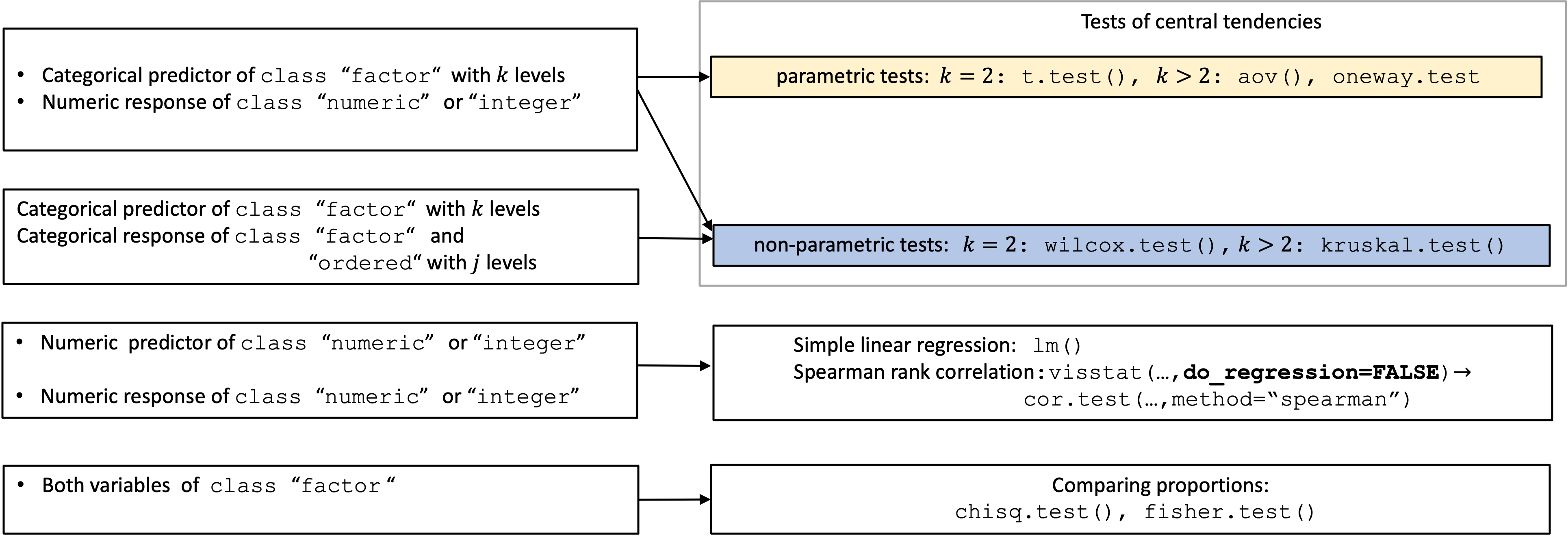
Figure 5.1: Overview of all implemented tests selected based on input class.

5.2 General linear model framework

Student’s t-test, Fisher’s ANOVA (both belonging to Route 1) and simple linear regression (in Route 3) are special cases of the general linear model framework (Thompson 2015) and share the same model assumptions: the expected value of the response is a linear function of the predictors, the error terms are mutually independent and normally distributed with expectation 0, and the error variance is constant.

Residuals are the empirical realisations of these error terms. To check whether the residuals fulfil the linear model assumptions, visstat() both visualises (see Section 5.2.3) and formally assesses the normality and homoscedasticity of the residuals by assumption tests (see Section 5.2.2) for tests belonging to Route 1 and Route 3. Note that only in Route 1, \(p\)-values derived from these assumption tests influence the test selection (Section 5.4.1).

Below, Section 5.2.1 formally defines the general linear model framework in the context of the implemented tests.

5.2.1 Model definition

In the general linear model, a response \(Y\) is modelled as a linear combination of \(k-1\) predictors \(x_j\). The general linear model for observation \(i,\;i = 1, \ldots, N\) is then

\[\begin{equation} \tag{5.1} Y_i = \beta_0 + \beta_1 x_{i1} + \cdots + \beta_{k-1} x_{i,k-1} + \varepsilon_i, \end{equation}\]

where \(Y_i\) is the response for observation \(i\), \(x_{ij}\) is the value of predictor \(j\) for observation \(i\), \(\beta_0, \beta_1, \ldots, \beta_{k-1}\) are the \(k\) parameters, and \(\varepsilon_i\) is the model error term. The model error terms \(\varepsilon_i\) are assumed to be independent and normally distributed with expectation 0 and constant variance \(\sigma^2\), in short \[\varepsilon_i \sim \mathscr{N}(0, \sigma^2), \quad\mathrm{mutually\; independent} \]

The variance \(\sigma^2\) represents the variation of the data about the regression, \(\operatorname{Var}(Y_i)=\operatorname{Var}(\varepsilon_i)=\sigma^2\), as both the (unknown) model parameters and predictors are not random.

From Eq. (5.1), the special cases used by visstat() follow from the predictor structure:

Student’s t-test uses one binary indicator variable \(x_{i1}\), with \(x_{i1}=0\) for group 1 and \(x_{i1}=1\) for group 2. Let \(\mu_1\) and \(\mu_2\) denote the expected mean values in the two population groups. For the expected values of the response, we then obtain \[E(Y_i \mid x_{i1}=0)=\mu_1=\beta_0\] for group 1 and \[E(Y_i \mid x_{i1}=1)=\mu_2=\beta_0+\beta_1\] for group 2. Testing \(H_0: \beta_1 = 0\) is therefore equivalent to testing \(H_0: \mu_1 = \mu_2\).

Fisher’s ANOVA generalises this coding to \(k-1\) binary indicator variables for \(k\) groups; testing \(H_0: \beta_1 = \cdots = \beta_{k-1} = 0\) is equivalent to testing equality of \(k\) group population means.

Simple linear regression uses one continuous predictor; \(H_0: \beta_1 = 0\) examines whether a linear relationship exists.

5.2.1.1 Residuals

The model error terms \(\varepsilon_i\) in Eq. (5.1) are not observed. Their observable counterparts are the residuals. After fitting the data with the corresponding linear model, the raw residual is

\[\begin{equation} e_i = y_i - \hat{y}_i, \tag{5.2} \end{equation}\]

where \(y_i\) is the observed value and \(\hat{y}_i\) the fitted value for observation \(i\);

\[\begin{equation} \hat{y}_i = b_0 + b_1 x_{i1} + \cdots + b_{k-1} x_{i,k-1} \end{equation}\] with the estimated values \(b_0, b_1, \ldots, b_{k-1}\) for the unknown model parameters \(\beta_0, \beta_1, \ldots, \beta_{k-1}\).

The magnitude of the raw residuals depends on the unknown model error variance \(\sigma^2\), which gets estimated by the square of the standard error \(SE_\text{res}^2 = \frac{\sum_{i=1}^{N} e_i^2}{N-k}\). Dividing the raw residuals by the standard error we obtain the z-residual

\[\begin{equation} z_i = \frac{e_i}{SE_\text{res}}, \tag{5.3} \end{equation}\]

which facilitates model comparison across different scales of the raw data.

5.2.1.1.1 Standardised residuals

The residual standard error \(SE_\text{res}\) is a global estimate for the unknown \(\sigma\), but not an estimate for the variance of the individual residual \(\operatorname{Var}(e_i)\). It can be shown (Cook and Weisberg 1982, 14; Schützenmeister et al. 2012, 145) that

\[\begin{equation} \operatorname{Var}(e_i)=\sigma^2(1-h_{ii}), \tag{5.4} \end{equation}\]

where the leverage \(h_{ii}\) of observation \(i\) is the \(i\)-th diagonal element of the \(N \times N\) hat matrix \(\mathbf{H}\) (Schützenmeister et al. 2012, 144), which maps the observed values onto the fitted values. \(h_{ii}\) measures how strongly observation \(i\)’s own observed value \(y_i\) influences its fitted value \(\hat{y}_i\).

Equation (5.4) shows that the raw residuals carry an unequal, leverage-dependent variance even when the errors are homoscedastic: observations with higher leverage have a smaller individual residual variance. Internally studentised (“standardised”) residuals correct for this artefact. Dividing \(e_i\) by its estimated individual standard error gives

\[\begin{equation} r_i =\frac{e_i}{\sqrt{ SE_\text{res}^2\,(1-h_{ii})}}= \frac{z_i}{\sqrt{1-h_{ii}}}. \tag{5.5} \end{equation}\]

5.2.2 General linear model assumption tests

Normality tests The normality of the standardised residuals is formally assessed using both the Shapiro–Wilk (SW) test (Shapiro and Wilk 1965; Royston 1982; Royston 1995) (shapiro.test(); Eq. (A.1)) and the Anderson–Darling test (Anderson and Darling 1952) (ad.test(); Eq. (A.2)). These tests offer complementary strengths: Anderson–Darling is highly sensitive to tail deviations in larger samples (Yap and Sim 2011), while Shapiro–Wilk generally exhibits greater power across non-normal distributions in small samples. Therefore in smaller samples, the Shapiro–Wilk test is used as the normality gate in the automated test selection (Section 5.4.1).

Homoscedasticity tests For grouped central-tendency analyses, variance homogeneity of standardised residuals (Cook and Weisberg 1982) is assessed using the package-implemented mean-centred Levene test (Levene 1960) (levene.test(); Eq. (A.3)) and Bartlett’s test (Bartlett 1937) (bartlett.test(); Eq. (A.4)). Bartlett’s test has greater power when normality holds, but the Levene test is more robust to departures from normality (missing citation) Therefore, Levene’s test is used as the variance gate in the automated workflow.

For simple linear regression, group-based variance tests are not applicable. There, visStatistics uses its package implementation bp.test() of the Breusch–Pagan test (Breusch and Pagan 1979) (Eq. (A.5)) on raw residuals (Schützenmeister et al. 2012).

5.2.3 Visualisation of the assumptions of the general linear model

Since algorithmic logic based on p-values of assumption tests cannot replace expert visual judgment, visstat() visualises the assumptions of the underlying linear model for the selection of tests of central tendency (Route 1) and for simple linear regression (correlation = FALSE) (Route 3).

For numeric responses with categorical predictors (Route 1), the diagnostic panel displays the residual histogram, the normal Q–Q plot with simultaneous tolerance band (STB) and point-wise tolerance band (TB) (Schützenmeister et al. 2012), and the absolute standardised residuals \(|r_i|\) (Eq. (5.5)) by group. The last panel shows whether residual spread is comparable across factor levels, the pattern assessed formally by the Levene (Eq. (A.3)) and Bartlett (Eq. (A.4)) variance checks.

For Route 3 (simple linear regression), the first two diagnostic panels follow the layout of Route 1, whereas the third panels displays z-scaled residuals versus fitted values.

The first row of the outer tile of the diagnostic plot reports p-values of residual-normality checks with the Shapiro–Wilk test and Anderson–Darling tests. The second row reports p-values of variance checks: Levene and Bartlett for grouped central-tendency analyses, or Breusch–Pagan for simple regression.

Note that among the displayed assumption tests, only the Shapiro–Wilk and Levene test results enter automated routing, and only in the central-tendency branch (see Section 5.4.1). Anderson–Darling, Bartlett, and Breusch–Pagan are diagnostic output only.

The Route 1 and Route 3 diagnostic-panel designs are illustrated in the examples in Figures 7.4, left, and 7.8, left.

5.3 Simulation results

The simulations focus on Route 1, the only branch in which visstat() lets assumption tests select the final test. The high-level problem is that grouped numeric data can answer two different questions. Parametric tests such as Student’s t-test, Fisher’s ANOVA, and their Welch variants test population means (Welch 1951; Rasch et al. 2011; Delacre et al. 2019). Rank-based tests such as Wilcoxon and Kruskal–Wallis test a rank-based distributional target and must not be interpreted as mean tests when distributional shapes differ (Fagerland and Sandvik 2009). An automated programme cannot know which question the user intends; therefore no single automatic default is correct in all cases (Fagerland and Sandvik 2009; Shatz 2024).

There are four coherent defaults. First, one can always stay within mean-based parametric testing. If this is the chosen estimand, a Welch default is defensible because it targets mean differences without requiring equal variances, avoids the operating-characteristic distortions introduced by preliminary variance tests (Moser and Stevens 1992; Zimmerman 2004; Rochon et al. 2012). Its cost is small in the equal-variance balanced case: Welch’s t-test coincides with Student’s t-test, and for more than two balanced groups the Welch ANOVA statistic converges to Fisher’s statistic with a relative difference of order \(n^{-1}\) (Eqs. (B.8) and (B.12)). In the four-group case used in the simulation, \(F/F_W = 1 + 3/[5(n-1)]\) (Eq. (B.13)) (Welch 1951; Rasch et al. 2011; Delacre et al. 2019). This keeps the estimand on the mean scale and gives directly interpretable estimates and confidence intervals (Jr 2026), but it can be weak for strongly skewed small samples (Blanca et al. 2017; Fagerland 2012) and can answer the wrong scientific question when the mean lies in a long tail (Fagerland and Sandvik 2009; Jr 2026). Second, one can let residual shape decide: if Shapiro–Wilk rejects residual normality, route to ranks; otherwise stay mean-based. This is transparent because the same diagnostic is displayed to the user, and Shapiro–Wilk has high power among normality tests in small to moderate samples (Razali and Wah 2011), but normality tests are underpowered in small samples and overpowered in large samples (Ghasemi and Zahediasl 2012; Fagerland 2012; Shatz 2024; Franc 2025). Third, one can combine both ideas by bypassing the normality gate above a sample-size threshold. This uses the Central Limit Theorem to protect mean-based inference (Lumley et al. 2002), but the threshold is necessarily shape- and design-dependent (Blanca et al. 2017; Fagerland 2012). Fourth, one can always use rank-based tests. This reduces distributional assumptions and can be efficient under skew (Bridge and Sawilowsky 1999; Jr 2026; Franc 2025), but changes the estimand (Fagerland and Sandvik 2009) and gives less direct mean-scale interpretation (Jr 2026).

The simulations below give the rationale for these design choices. They do not prove a universally best route; they show the price and benefit of each automatic compromise. Abbreviations used throughout are: F = Fisher’s ANOVA; W = Welch’s heteroscedastic ANOVA; L = Levene gate selecting F or W; KW = Kruskal–Wallis; SW = Shapiro–Wilk gate selecting W or KW; and SW+L = Shapiro–Wilk gate selecting KW or, if the mean branch is retained, L.

The current code fits a group model, tests the standardised residuals, and uses the Shapiro–Wilk result as the first gate: rejected residual normality routes to Wilcoxon or Kruskal–Wallis; retained residual normality keeps the result in the mean-based branch. The design question is therefore specific: should the parametric side of the Shapiro–Wilk gate default directly to Welch (SW), or should it include the Levene gate (SW+L) and select Fisher/Student only when homoscedasticity is not rejected?

Rochon et al. (Rochon et al. 2012) is used only as background here: two-stage testing can change conditional error rates, so the final procedure must be judged by its simulated final-test rejection rates. The figures below separate three questions. The first Type I simulation checks whether the candidate routes keep the nominal rejection rate when both the equal-means and rank-distribution nulls are true. The second keeps the equal-means null true but violates equality of distributions, so F, W, and L remain mean-null tests while SW and SW+L become final-test rejection rates after possible hypothesis switching. The power simulation then asks how the routes behave under real ordered group differences.

The simulation layout follows the competitor logic. Blanca et al. (Blanca et al. 2017) assess Fisher’s ANOVA under zero group effect, non-normal distributions, balanced and unbalanced group sizes, and Bradley’s robustness criterion. Delacre et al. (Delacre et al. 2019) cross sample-size ratios, SD ratios, and sample-size/SD pairings to compare Fisher-type and Welch-type ANOVA. Fagerland and Sandvik (Fagerland and Sandvik 2009) separate the equal-means target from rank-based targets and show why rank tests must not be read as mean tests when distributional shapes differ. We therefore use two Type I settings: identical distributions, where both the equal-means and equal-rank-distribution nulls are true, and equal means with unequal distributions, where only the equal-means null is the common target for F, W, and L.

The normal input is the standard normal distribution, \(X \sim \mathcal{N}(0,1)\): mean 0, variance 1, skewness 0, and kurtosis 3. Excess kurtosis is kurtosis minus 3, so it is 0 for the standard normal distribution. Gamma input follows the standardised Gamma path. For \(X \sim \Gamma(\alpha,\theta)\), with shape parameter \(\alpha>0\) and scale parameter \(\theta>0\), the mean is \(E(X)=\alpha\theta\), the variance is \(\mathrm{Var}(X)=\alpha\theta^2\), the skewness is \(2/\sqrt{\alpha}\), and the kurtosis is \(3+6/\alpha\). The excess kurtosis is therefore \(6/\alpha\) (Forbes et al. 2010, 109). In the simulations \(\theta=1\), \(\alpha\in\{16,4,1,0.25\}\), and draws are standardised by \(Z=(X-\alpha\theta)/(\theta\sqrt{\alpha})\). Thus the Gamma columns deliberately vary skewness and excess kurtosis together.

The Type I simulations use four groups and \(B=50{,}000\) Monte Carlo replications per cell. For an estimated rejection probability \(\hat p\), the Monte Carlo standard error is \[ SE_{\mathrm{MC}}=\sqrt{\hat p(1-\hat p)/B}. \] This is about 0.10 percentage points at \(\hat p=0.05\), with a maximum of about 0.22 percentage points at \(\hat p=0.50\).

The first setting is the clean null case. All groups have the same population mean and the same distribution; therefore the equal-means null is true for F, W, and L, and the rank-distribution null is also true for KW. This is the only Type I figure where standalone KW is a valid comparator.

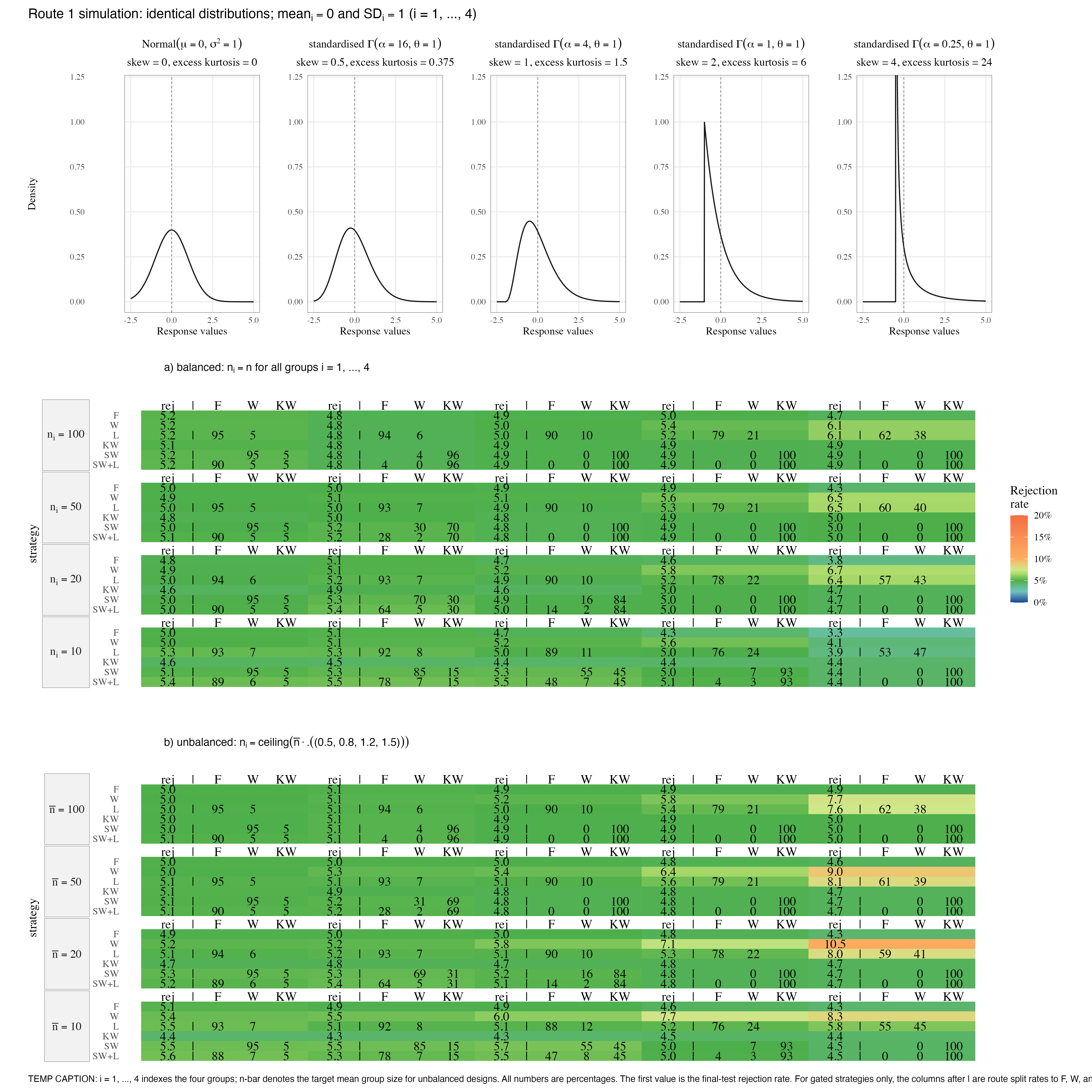
Figure 5.2: Route 1 Type I simulation under identical distributions and identical means. The heatmap reports final-test rejection rates at alpha = 5%. Green marks Bradley’s 2.5%–7.5% interval. Cells for SW and SW+L additionally report the route split.

Across the identical-distribution cells, SW and SW+L remain inside Bradley’s interval. Their mean final-test rejection rates are 5.01% and 5.03%, respectively. The important point is not that SW fails to route to KW under skew; it does route to KW. The point is that this does not create false rejection here, because the rank-distribution null is true as well.

Table 5.1: Summary of the identical-distribution Type I simulation by distribution shape. Entries are ranges across the displayed n-regimes.

Distribution	Skewness	Excess kurtosis	F	W	L	KW	SW	SW+L	SW to W	SW to KW	SW+L to F	SW+L to W	SW+L to KW
normal, mean = 0, SD = 1	0	0	4.8%–5.2%	4.9%–5.4%	5.0%–5.5%	4.4%–5.1%	5.0%–5.5%	5.0%–5.6%	94.8%–95.2%	4.8%–5.2%	88.2%–90.1%	5.0%–7.0%	4.8%–5.2%
standardised Gamma, alpha = 16	0.5	0.375	4.8%–5.1%	4.8%–5.5%	4.8%–5.3%	4.3%–5.1%	4.8%–5.5%	4.8%–5.5%	4.3%–85.0%	15.0%–95.7%	4.0%–78.0%	0.3%–7.2%	15.0%–95.7%
standardised Gamma, alpha = 4	1	1.5	4.7%–5.0%	5.0%–6.0%	4.9%–5.1%	4.3%–4.9%	4.8%–5.7%	4.8%–5.5%	0.0%–55.0%	45.0%–100.0%	0.0%–47.6%	0.0%–7.7%	45.0%–100.0%
standardised Gamma, alpha = 1	2	6	4.3%–5.0%	5.4%–7.7%	5.0%–5.6%	4.4%–5.0%	4.8%–5.0%	4.8%–5.1%	0.0%–7.4%	92.6%–100.0%	0.0%–4.1%	0.0%–3.4%	92.6%–100.0%
standardised Gamma, alpha = 0.25	4	24	3.3%–4.9%	4.1%–10.5%	3.9%–8.1%	4.4%–5.0%	4.4%–5.0%	4.4%–5.0%	0.0%	100.0%	0.0%	0.0%	100.0%

The second Type I setting is the mean-null stress test. The group means are equal, but the group distributions differ through the standard-deviation design. Therefore F, W, and L still assess the equal-means null, but KW is not a standalone Type I comparator for that null. SW and SW+L are retained in the figure because they are the actual automatic procedures; their cells report the rejection rate of the final selected test after a possible switch to KW.

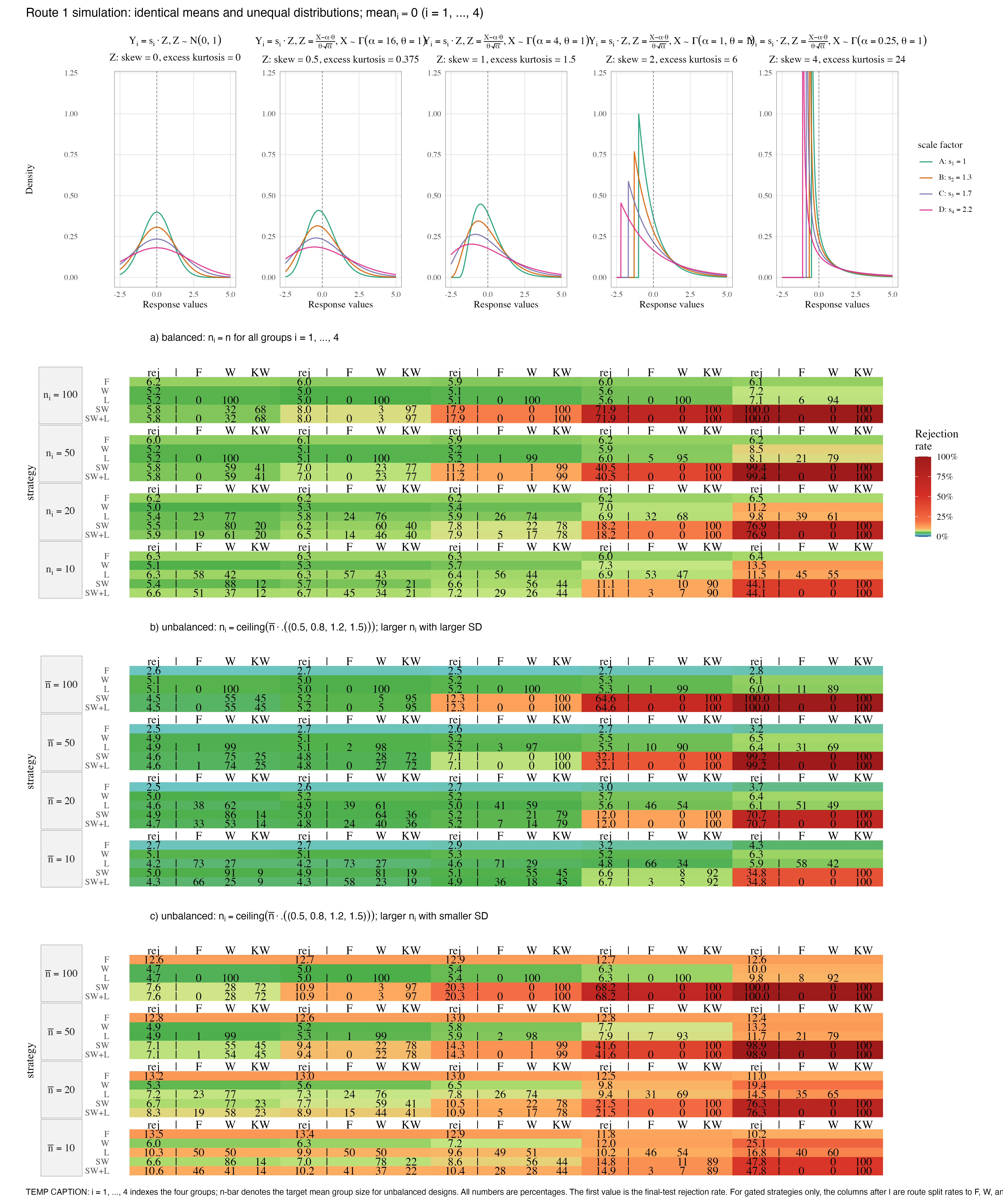
Figure 5.3: Route 1 equal-means simulation with unequal group distributions. F, W, and L are mean-null tests; SW and SW+L report final-test rejection after possible routing to Kruskal–Wallis.

Read strictly as equal-means testing, Welch is the most stable of the mean-based strategies in this simulation: the mean rejection rates are F = 7.20%, W = 6.81%, and L = 6.70%. SW and SW+L are much higher, 27.15% and 27.39%, because the Shapiro–Wilk gate often switches to KW. This is the central interpretation: SW and SW+L are method switches, not better equal-means tests.

Table 5.2: Summary of the unequal-distribution Type I simulation by distribution shape. Entries are ranges across the unequal-distribution n/SD regimes.

Distribution	Skewness	Excess kurtosis	F	W	L	SW	SW+L	SW to W	SW to KW	SW+L to F	SW+L to W	SW+L to KW
normal, mean = 0, SD = 1	0	0	2.5%–13.5%	4.7%–6.0%	4.2%–10.3%	4.5%–7.6%	4.3%–10.6%	27.6%–90.5%	9.5%–72.4%	0.0%–65.8%	24.8%–73.9%	9.5%–72.4%
standardised Gamma, alpha = 16	0.5	0.375	2.6%–13.4%	5.0%–6.3%	4.2%–9.9%	4.8%–10.9%	4.3%–10.9%	3.1%–81.0%	19.0%–96.9%	0.0%–57.6%	3.1%–46.2%	19.0%–96.9%
standardised Gamma, alpha = 4	1	1.5	2.5%–13.0%	5.1%–7.2%	4.6%–9.6%	5.1%–20.3%	4.9%–20.3%	0.0%–56.1%	43.9%–100.0%	0.0%–36.1%	0.0%–28.1%	43.9%–100.0%
standardised Gamma, alpha = 1	2	6	2.7%–12.8%	5.2%–12.0%	4.8%–10.2%	6.6%–71.9%	6.7%–71.9%	0.0%–10.6%	89.4%–100.0%	0.0%–3.3%	0.0%–7.2%	89.4%–100.0%
standardised Gamma, alpha = 0.25	4	24	2.8%–12.6%	6.1%–25.1%	5.9%–16.8%	34.8%–100.0%	34.8%–100.0%	0.0%–0.1%	99.9%–100.0%	0.0%	0.0%–0.1%	99.9%–100.0%

The power simulation addresses the complementary question: if real ordered group differences exist, how much power is lost or gained by SW and SW+L? This completed power simulation is balanced and homoscedastic, with four group means shifted by 0, 0.25, 0.50, and 0.75 after standardisation.

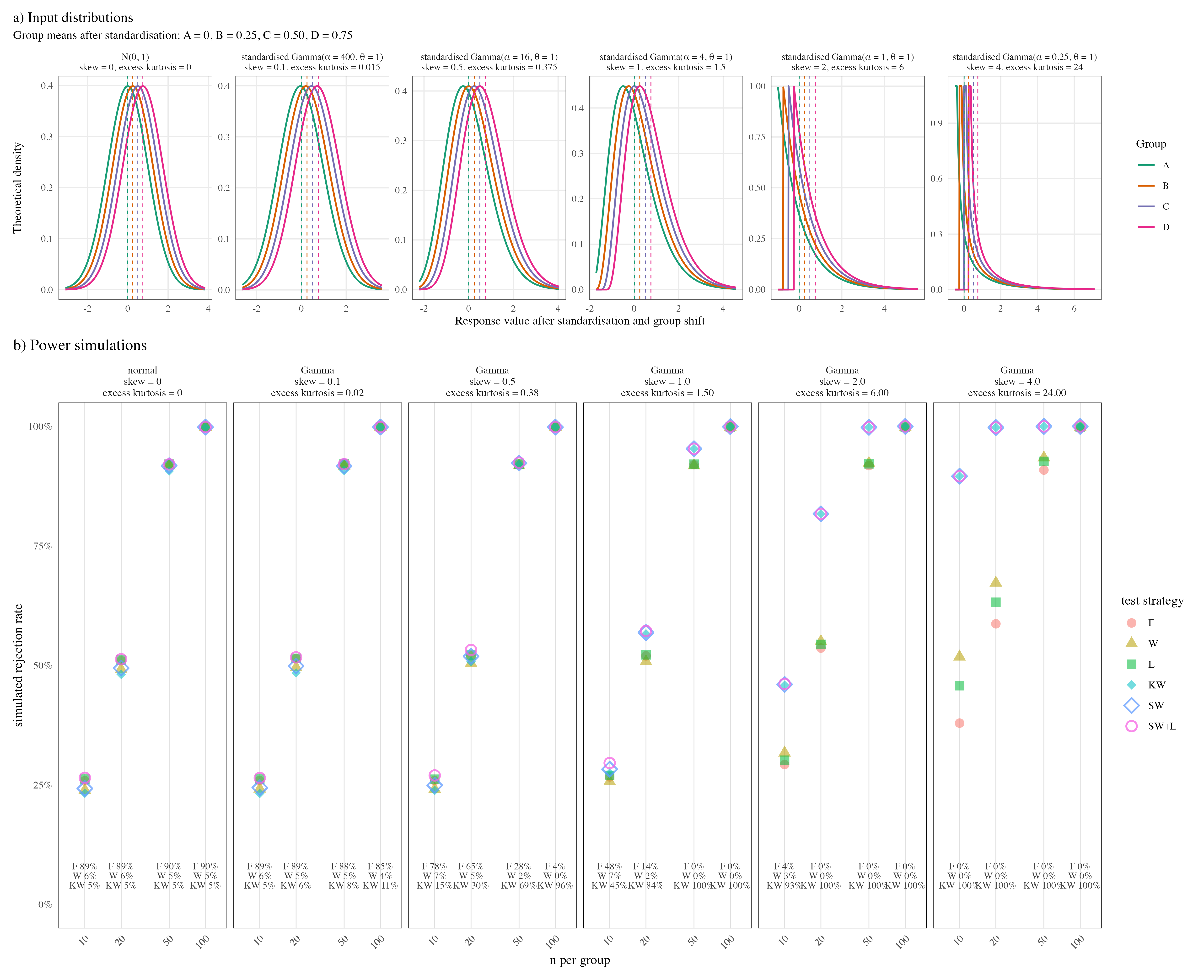
Figure 5.4: Power simulation. (a) Theoretical input distributions. Group A has mean 0 after standardisation; groups B–D are shifted by 0.25, 0.50, and 0.75. (b) Power simulations for six testing strategies based on 50,000 Monte Carlo draws per setting from the population densities depicted in (a). F, W, and L are mean-based strategies and test equality of means; KW is rank-based and tests equality of rank distributions. SW and SW+L are routed strategies, so their tested null hypothesis depends on the selected final test. The F, W, and KW percentages printed inside the lower panels give the proportions of simulations routed by SW+L to Fisher, Welch, and Kruskal–Wallis, respectively.

Around normality and mild Gamma skew, SW+L has slightly higher power than SW because the Levene gate sometimes retains Fisher in homoscedastic data. At stronger skew, both SW and SW+L route almost entirely to KW and their power is practically identical.

Table 5.3: Summary of the power simulation by distribution shape. Power entries are means across n = 10, 20, 50, 100, and 200; the figure shows the n-specific values.

Distribution	Skewness	Excess kurtosis	F	W	L	KW	SW	SW+L	SW+L regret	SW to W	SW to KW	SW+L to F	SW+L to W	SW+L to KW
normal, mean = 0, SD = 1	0	0	73.8%	73.0%	73.9%	72.4%	73.1%	73.9%	0.01%	94.9%–95.2%	4.8%–5.1%	88.7%–90.1%	4.8%–6.5%	4.8%–5.1%
standardised Gamma, alpha = 400	0.1	0.015	73.9%	73.1%	73.9%	72.5%	73.2%	74.0%	0.01%	83.8%–94.8%	5.2%–16.2%	79.4%–88.8%	4.4%–6.2%	5.2%–16.2%
standardised Gamma, alpha = 16	0.5	0.375	74.0%	73.3%	74.1%	73.3%	73.8%	74.5%	0.00%	0.0%–84.7%	15.3%–100.0%	0.0%–77.8%	0.0%–6.9%	15.3%–100.0%
standardised Gamma, alpha = 4	1	1.5	74.1%	73.6%	74.2%	75.9%	76.1%	76.4%	0.00%	0.0%–55.1%	44.9%–100.0%	0.0%–47.7%	0.0%–7.4%	44.9%–100.0%
standardised Gamma, alpha = 1	2	6	74.9%	75.8%	75.3%	85.5%	85.5%	85.5%	0.00%	0.0%–7.4%	92.6%–100.0%	0.0%–4.1%	0.0%–3.3%	92.6%–100.0%
standardised Gamma, alpha = 0.25	4	24	77.4%	82.5%	80.3%	97.9%	97.9%	97.9%	0.00%	0.0%	100.0%	0.0%	0.0%	100.0%

Finally, the normal homoscedastic corner of Figure 5.4 is summarised in Table 5.4. This small advantage of Fisher/Student is exactly the balanced equal-variance corner quantified in Eq. (B.13): in the four-group simulation, \(F/F_W = 1 + 3/[5(n-1)]\), so the statistic-level difference is of order \(n^{-1}\). This is not an argument for variance pretesting. The literature separates the two issues: Welch-type tests are recommended as unconditional mean tests when equal variances are doubtful (Welch 1951; Rasch et al. 2011; Delacre et al. 2019), whereas choosing Student/Fisher or Welch after a preliminary variance test is discouraged because the selection step changes the operating characteristics of the final test (Moser and Stevens 1992; Zimmerman 2004; Rochon et al. 2012).

Table 5.4: Fisher/Welch comparison in the normal homoscedastic corner of the power simulation.

n	F/F_W theory	F power	W power	L power	SW+L to F	SW+L to W	SW+L to KW
10	1.0667	25.9%	23.9%	26.2%	88.7%	6.5%	4.8%
20	1.0316	51.0%	49.2%	51.1%	89.5%	5.5%	5.0%
50	1.0122	92.1%	91.8%	92.1%	90.1%	5.0%	4.9%
100	1.0061	99.9%	99.9%	99.9%	90.1%	4.9%	5.0%
200	1.0030	100.0%	100.0%	100.0%	90.1%	4.8%	5.1%

The only remaining reason for SW+L is therefore not statistical optimality for the equal-means null, but consistency with the displayed model. Route 1 shows the residual diagnostics of the equal-variance Gaussian group model; if both displayed GLM assumptions pass, keeping Fisher/Student available makes the reported test correspond to the model just diagnosed. If that design link is not wanted, the literature and these simulations both favour the simpler SW route: Shapiro–Wilk retained means Welch, Shapiro–Wilk rejected means Kruskal–Wallis.

If Route 1 is read strictly as an equal-means machine, the simulations support Welch as the clean default. If Route 1 is allowed to use residual shape as a method switch, SW is the simpler automatic route. SW+L is a model-display compromise: it preserves the Fisher/Student GLM branch when both residual normality and homoscedasticity are retained, but its Type I error cost must be read from the Type I simulations, not from the Fisher/Welch power comparison.

Thus the simulations do not prove that SW+L is the best equal-means procedure. They show the price and benefit of the automatic route. The price is that, under equal means but unequal distributions, SW and SW+L often report the rejection rate of KW after the hypothesis has changed. The benefit is that the switch is visible and diagnostic-driven. The final design decision is therefore not statistical optimality in the abstract, but which default the package wants to make explicit: Welch for fixed equal-means inference, SW for a parsimonious shape-based switch, or SW+L for the same switch while preserving the GLM Fisher/Student branch when its displayed assumptions pass.

5.4 Route-specific decision rules

The general branching is driven by input class and factor levels (Section 5.1). Within the selected route, additional rules determine the selected test and output; these route-specific rules are detailed below.

5.4.1 Route 1: Numeric response, categorical predictor

A numeric response with a categorical predictor with \(k\) “levels” (in the following “groups”) asks whether the response differs between groups.

Figure 5.5 expands the routing logic for tests of central tendencies.

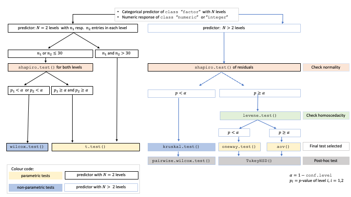
Figure 5.5: Decision tree for tests of central tendency. If all group-specific sample sizes are greater than 50, the formal residual normality test is bypassed and variance homogeneity is assessed directly. Otherwise, Shapiro–Wilk on model residuals determines whether the route remains mean-based or switches to rank-based tests; the Levene test then selects equal-variance or Welch-type procedures.

The first split checks group size:

From Shatz “When violations are detected, the diagnostics can also drive the decision of what to do; common options include switching methods (e.g., to robust non-parametric ones), transforming the data (e.g., by taking its logarithm), or sticking to the original analysis (Casson & Farmer, 2014; Pek et al., 2018; Pole & Bondy, 2012; Vallejo et al., 2021).”

The literature question is separate: Fisher/Welch can still be robust to that non-normality, especially with adequate sample size. So the gate may be assumption-correct but not always necessary.

This avoids switching to rank-based tests because of negligible residual-normality deviations in large samples (Ghasemi and Zahediasl 2012; Shatz 2024).

A linear model of Eq. (5.1) is fitted between the numeric response and the categorical predictor, and the model residuals of Eq. (5.2) are extracted.

The Shapiro–Wilk (SW) normality test is then applied as the residual-normality gate, because simulation studies report high power for small to moderate sample sizes (Razali and Wah 2011).

If the SW-test rejects residual normality (\(p_\text{SW} \le \alpha\)), robust non-parametric tests are selected: wilcox.test() (Eq. (C.1)) for two groups, or kruskal.test() (Eq. (C.2)) followed by Holm-adjusted pairwise.wilcox.test() for more than two groups.

If residual normality is not rejected or not tested in larger samples, variance homogeneity is assessed with the mean-centred Levene test (L) (Levene 1960) (Eq. (A.3)).

For homoscedastic data (\(p_\text{L} > \alpha\)), t.test(var.equal = TRUE) (Eq. (B.1)) is applied for two groups, or Fisher’s aov() (Eq. (B.2)) for more than two groups. For heteroscedastic data (\(p_\text{L} \le \alpha\)), Welch’s t.test() (Eq. (B.4)) is applied for two groups, or Welch’s oneway.test() (Eq. (B.6)) for more than two groups.

A type I error of the Levene test merely routes homoscedastic data to Welch’s t-test or Welch’s one-way ANOVA, which lose only negligible power when variances are in fact equal simple sizes are large. (Rasch et al. 2011; Delacre et al. 2019).

Post-hoc tests

ANOVA, Welch ANOVA, and Kruskal–Wallis are omnibus tests: a significant test result tells us that some group differs, but not which.

To identify the differing pairs, visstat() tests all pairwise comparisons among the factor levels, defining a family of tests. Because the three omnibus tests rest on different assumptions, each branch uses a matching post-hoc procedure:

• TukeyHSD() (Eq. (B.3)) after aov() controls the family-wise error rate through the studentised range distribution under a common-variance assumption.

• games.howell() (Eq. (B.7)) after oneway.test() uses separate variance estimates and Welch-adjusted degrees of freedom for each pair, making it the appropriate post-hoc procedure for the heteroscedastic Welch branch.

• pairwise.wilcox.test(p.adjust.method = "holm") after kruskal.test() uses Holm’s step-down adjustment for the pairwise Wilcoxon tests in the Kruskal–Wallis branch.

The graphical results panel of these omnibus tests consists of box plots (see examples in Section 7.1) enriched with significance letters to visualise the post-hoc analysis: Pairs whose adjusted post-hoc \(p\)-value falls below \(\alpha\) are marked with different green significance letters below the box plots; pairs sharing a letter are not significantly different.

5.4.2 Route 2: Ordered response

An ordered categorical response with a categorical predictor or ordered categorical predictor is treated as a rank-based group comparison. The ordered response is converted to integer level codes and analysed with the Wilcoxon rank-sum test for two groups or the Kruskal–Wallis test for more than two groups.

5.4.3 Route 3: Numeric response, numeric predictor

Two numeric variables ask whether a numeric response changes with a numeric predictor. By default, visstat() fits a simple linear regression (Eq. (7.1)). and the diagnostic panel described in Section 5.2.3 is displayed. If general linear model assumptions are violated, the corresponding p-values trigger warnings and recommendations, but no automatic model replacement. The regression output is shown in Section 7.3.1.

5.4.4 Route 4: Two unordered factors

Two unordered factors ask whether two categorical variables are independent. visstat() uses Pearson’s \(\chi^2\) test or Fisher’s exact test, depending on expected cell counts following Cochran’s rule (Cochran 1954): the \(\chi^2\) approximation is used if no expected cell count is less than 1 and no more than 20% of cells have expected counts below 5. Yates’ continuity correction is applied by default to \(2 \times 2\) tables when the \(\chi^2\) approximation is used.

5.4.5 Optional rank-correlation mode

The four routes above describe the default, automatic test selection behaviour. For ordered–ordered and numeric–numeric input vectors, the user can instead request a rank-correlation analysis by setting correlation = TRUE.

Both optional analyses test monotone association and are computed by cor.test(): Kendall’s \(\tau_b\) (Eq. (E.1)) with method = "kendall", exact = FALSE for two ordered variables, and Spearman’s \(\rho\) (Eq. (E.2)) with method = "spearman" for two numeric variables. Kendall’s \(\tau_b\) corrects for ties present with few ordered levels (Agresti 2010; Xu et al. 2013).

Note that for numeric–numeric input, Pearson correlation is not implemented as a separate optional mode as in simple linear regression with an intercept, the two-sided test of zero slope and the two-sided Pearson correlation test return the same \(p\)-value.

5.5 Reported p-values and effect sizes

The selected test output includes the p-value for the corresponding null hypothesis. As a complementary output component, the effect_size field reports the effect-size name, numeric estimate, and method description.

The exported package function effect_size() computes these estimates; implemented formulae are given in Appendix F.

The p-value quantifies evidence against the null hypothesis, whereas the effect-size estimate describes the magnitude of the selected comparison, association, or model fit on the scale defined in Appendix F (Fritz et al. 2012; Levine and Hullett 2002).

6 The visstat methods

Objects returned by visstat() are of class "visstat" and support the S3 methods print(), summary(), and plot(). Each is demonstrated on a worked object in Section 7.1.1.2.

• print() lists the returned components.
• summary() prints the full returned object, including assumption tests, post-hoc comparisons, confidence level, and effect_size where available.
• plot() lists the available plots by default; with which, it either replays a captured plot (in an interactive R session) or reports the selected saved file path.

6.1 Saved graphics

When visstat() is called with graphicsoutput specified, plot() lists the generated file paths instead. All generated graphics can be saved in any file format supported by Cairo() (Urbanek and Horner 2025), including “png”, “jpeg”, “pdf”, “svg”, “ps”, and “tiff”. If plotName is provided, the main result plot uses this name. The assumption-diagnostic plot adds the prefix "glm_assumptions_". If plotName is not provided, file names are generated from the selected plot type and the input variable names.

7 Usage and Examples

The examples follow the routes outlined in Section 5.1 and are chosen to trigger every branch.

Within the group-comparison routes, examples are ordered such that the two-group case is followed by its generalisation to more than two groups: Student’s t-test by Fisher’s one-way ANOVA, Welch’s t-test by Welch’s one-way ANOVA, and Wilcoxon rank-sum by Kruskal–Wallis.

Where needed, the example descriptions add interpretive details on the graphical output, such as significance letters, regression bands, or mosaic plots.

7.1 Route 1: Numeric response, categorical predictor

7.1.1 Student’s t-test and Fisher’s one-way ANOVA

7.1.1.1 Student’s t-test

The ToothGrowth dataset records odontoblast length in 60 guinea pigs given vitamin C by orange juice (OJ) or ascorbic acid (VC). With delivery method as predictor and length as response, the assumption-diagnostic panel shows no residual-normality or variance-homogeneity violation. visstat() therefore selects Student’s t-test, and the result panel shows the two-group box plot with the selected test result.

student_ttest <- visstat(ToothGrowth$supp, ToothGrowth$len)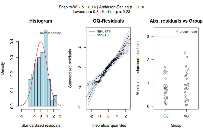

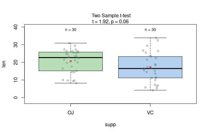
Figure 7.1: Student’s t-test applied to the ToothGrowth dataset (len vs. supp). Assumption diagnostics (Shapiro–Wilk does not reject residual normality; Levene does not reject residual variance homogeneity) select the equal-variance mean-based path, followed by box plots with the Student t-test result.

7.1.1.2 Fisher’s one-way ANOVA with Tukey HSD post-hoc comparisons with methods demonstration

The PlantGrowth dataset records yields (as measured by dried weight of plants) for a control group and two treatment groups. This dataset serves a double purpose: it demonstrates both a branching result and the visstat() S3 methods print(), summary(), and plot() (Section 6).

anova_plantgrowth <- visstat(PlantGrowth$group, PlantGrowth$weight)

In this branch visstat() generates two plots: the assumption-diagnostic panel (which = 1) and the result panel with box plots and post-hoc significance letters (which = 2). Calling plot() without which first lists both available plots:

plot(anova_plantgrowth)

## Plot [1] captured. Use plot(obj, which = 1) to display.

## Plot [2] captured. Use plot(obj, which = 2) to display.

Figure 7.2(a) replays the assumption-diagnostic panel (which = 1). With control and treatment groups as predictor and plant weight as response, Shapiro–Wilk does not reject normality of the model residuals and levene.test() does not reject homoscedasticity, so visstat() takes the equal-variance mean-based path. Figure 7.2(b) replays the result panel (which = 2).

plot(anova_plantgrowth, which = 1)
plot(anova_plantgrowth, which = 2)

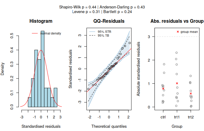
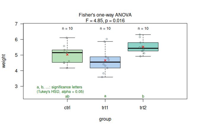
Figure 7.2: PlantGrowth Fisher’s one-way ANOVA (weight vs. group). (a) Assumption-diagnostic panel. (b) Result panel with Tukey HSD significance letters (\(\alpha = 0.05\)).

The omnibus F-test is significant at \(\alpha = 0.05\), and the Tukey HSD post-hoc comparison finds no significant difference between the control group and either treatment, but the difference between trt1 and trt2 is significant.

To save the graphics, call visstat() with graphicsoutput; the file paths are returned in the "plot_paths" attribute. Here, plotName is set explicitly so that the output names are stable.

anova_plantgrowth_stored <- visstat(
  PlantGrowth$group,
  PlantGrowth$weight,
  graphicsoutput = "png",
  plotName = "anova_plantgrowth",
  plotDirectory = tempdir()
)
paths <- attr(anova_plantgrowth_stored, "plot_paths")
print(basename(paths))

## [1] "glm_assumptions_anova_plantgrowth.png"
## [2] "anova_plantgrowth.png"

print() lists the returned components:

print(anova_plantgrowth)

## Object of class 'visstat'
## 
## Available components:
## [1] "summary statistics of ANOVA" "post-hoc analysis "         
## [3] "conf.level"                  "effect_size"

summary() prints the full object, including assumption tests, post-hoc comparisons, and effect size.

summary(anova_plantgrowth)

## Summary of visstat object
## 
## --- Named components ---
## [1] "summary statistics of ANOVA" "post-hoc analysis "         
## [3] "conf.level"                  "effect_size"                
## 
## --- Contents ---
## 
## $summary statistics of ANOVA:
##             Df Sum Sq Mean Sq F value Pr(>F)  
## fact         2  3.766  1.8832   4.846 0.0159 *
## Residuals   27 10.492  0.3886                 
## ---
## Signif. codes:  0 '***' 0.001 '**' 0.01 '*' 0.05 '.' 0.1 ' ' 1
## 
## $post-hoc analysis :
##   Tukey multiple comparisons of means
##     95% family-wise confidence level
## 
## Fit: aov(formula = samples ~ fact)
## 
## $fact
##             diff        lwr       upr     p adj
## trt1-ctrl -0.371 -1.0622161 0.3202161 0.3908711
## trt2-ctrl  0.494 -0.1972161 1.1852161 0.1979960
## trt2-trt1  0.865  0.1737839 1.5562161 0.0120064
## 
## 
## $conf.level:
## [1] 0.95
## 
## $effect_size:
## $name
## [1] "omega-squared"
## 
## $estimate
## [1] 0.2040788
## 
## $effect_size_method
## [1] "Omega-squared for one-way ANOVA"

7.1.2 Welch’s t-test and Welch’s one-way ANOVA

7.1.2.1 Welch’s t-test

The Motor Trend Car Road Tests dataset (mtcars) contains 32 observations, where mpg denotes miles per (US) gallon and am represents the transmission type (0 = automatic, 1 = manual). With binary factor am and continuous response mpg, the assumption-diagnostic panel shows that Shapiro–Wilk does not reject normality of the model residuals, while the Levene test detects heteroscedasticity. The routing therefore leads to Welch’s t-test rather than Student’s t-test, and the result panel shows the corresponding two-group comparison.

mtcars$am <- as.factor(mtcars$am)
t_test_stats <- visstat(mtcars$am, mtcars$mpg)

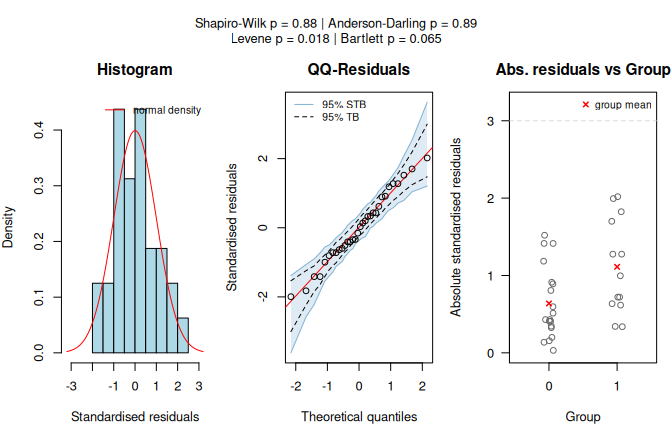
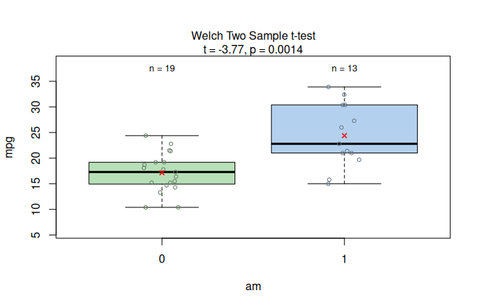
Figure 7.3: Welch’s t-test applied to the mtcars dataset (mpg vs. am). Assumption diagnostics (Shapiro–Wilk does not reject residual normality; Levene rejects residual variance homogeneity) select the unequal-variance mean-based path, followed by box plots with the Welch t-test result.

7.1.2.2 Welch’s heteroscedastic one-way ANOVA with Games–Howell post-hoc comparisons

In the iris dataset, using Species as predictor and Sepal.Length as response, the assumption-diagnostic panel shows that Shapiro–Wilk does not reject normality of the model residuals, whereas the Levene test rejects homoscedasticity at the given \(\alpha = 5\%\). visstat() therefore selects Welch’s heteroscedastic one-way ANOVA (oneway.test()) and applies Games–Howell post-hoc comparisons. The result panel shows the box plots and Games–Howell significance letters.

welch_anova_iris <- visstat(iris$Species, iris$Sepal.Length)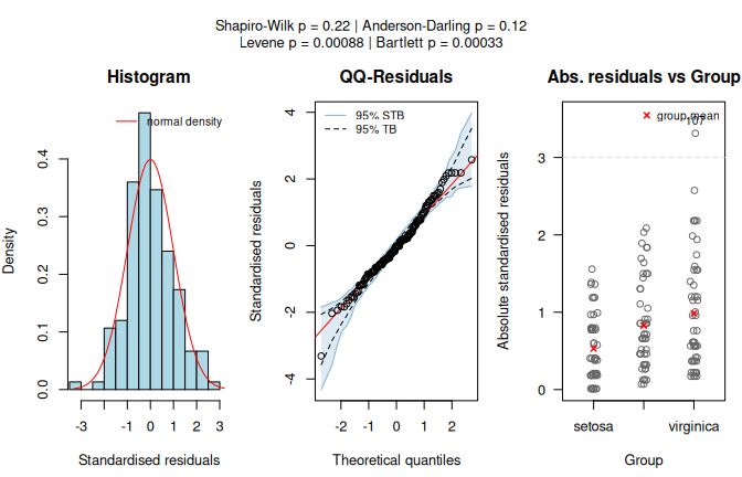

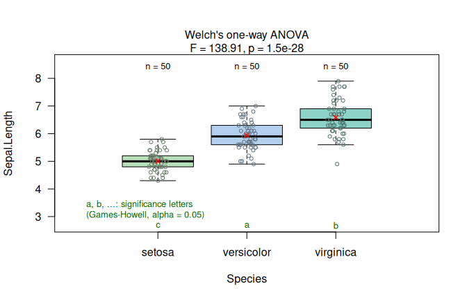
Figure 7.4: Welch’s heteroscedastic one-way ANOVA applied to the iris dataset (Sepal.Length vs. Species). Assumption diagnostics (Shapiro–Wilk does not reject residual normality; Levene rejects residual variance homogeneity) select the unequal-variance mean-based path, followed by box plots with Games–Howell significance letters (\(\alpha = 0.05\)).

7.1.3 Wilcoxon rank-sum test and Kruskal–Wallis test

7.1.3.1 Wilcoxon rank-sum test

The warpbreaks dataset records thread breaks during weaving. Using wool type (A or B) as predictor and the number of breaks as response, the assumption-diagnostic panel shows that the Shapiro–Wilk test rejects normality of the model residuals. visstat() therefore selects the Wilcoxon rank-sum test, and the result panel shows the rank-based two-group comparison.

wilcoxon_stats <- visstat(warpbreaks$wool, warpbreaks$breaks)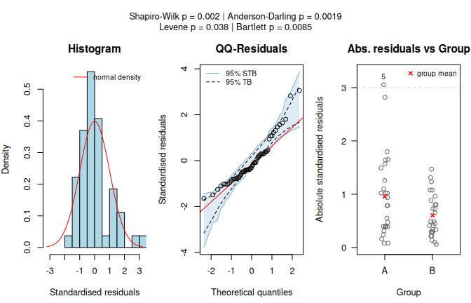

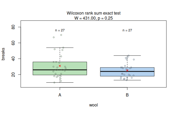
Figure 7.5: Wilcoxon rank-sum test applied to the warpbreaks dataset (breaks vs. wool). Assumption diagnostics (Shapiro–Wilk rejects residual normality; non-parametric path selected) and box plots with the Wilcoxon test result.

7.1.3.2 Kruskal–Wallis rank sum test with pairwise Wilcoxon post-hoc comparisons

In the iris data set, Petal.Width by Species follows a different route than Sepal.Length by Species above (Figure 7.4), because the assumption diagnostics differ. The assumption-diagnostic panel shows clear departures from normality, and both normality tests return very small \(p\)-values. Since Shapiro–Wilk falls below \(\alpha\), visstat() switches to kruskal.test() followed by Holm-adjusted pairwise.wilcox.test(). The result panel shows the box plots and Holm-adjusted significance letters; all three species differ significantly in petal width, as indicated by distinct letters.

kruskal_iris <- visstat(iris$Species, iris$Petal.Width)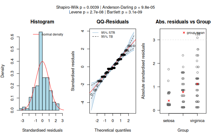

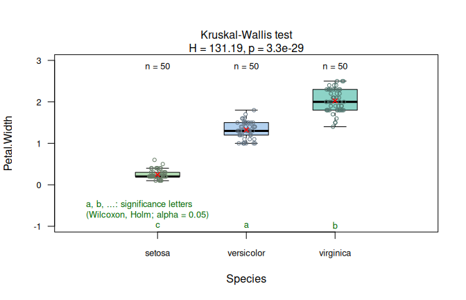
Figure 7.6: Kruskal-Wallis test applied to the iris dataset (Petal.Width vs. Species). Assumption diagnostics (Shapiro–Wilk rejects residual normality; non-parametric path selected) and box plots with Holm-adjusted pairwise Wilcoxon significance letters (\(\alpha = 0.05\)).

7.2 Route 2: Ordered response

7.2.1 Ordered response, categorical factor

7.2.1.1 Wilcoxon rank-sum test with ordered response

The Titanic dataset contains passenger counts by, among other variables, passenger class and gender. After expanding the table to individual rows, passenger class is treated as ordered and gender as a two-level predictor. visstat() selects the Wilcoxon rank-sum test. The result panel therefore displays the rank-test comparison on the numeric level scores (see Figure 7.7, left).

titanic_df <- counts_to_cases(as.data.frame(Titanic))
titanic_df$Class <- ordered(titanic_df$Class,
                            levels = c("1st", "2nd", "3rd", "Crew"))
wilcox_ordered <- visstat(titanic_df$Sex, titanic_df$Class)

## Warning: Ordered response detected. Converting to integer level codes for
## non-parametric analysis.

7.2.1.2 Kruskal–Wallis test with ordered response

With three predictor groups, visstat() routes to kruskal.test() followed by Holm-adjusted pairwise.wilcox.test(). The result panel shows the Kruskal–Wallis comparison and Holm-adjusted significance letters on the numeric level scores (see Figure 7.7, right). A synthetic survey records perceived car comfort on a five-point scale across three markets.

set.seed(123)
market <- factor(rep(c("Europe", "North America", "Asia"), each = 50))
comfort_numeric <- c(
  sample(1:5, 50, replace = TRUE, prob = c(0.30, 0.30, 0.20, 0.15, 0.05)),
  sample(1:5, 50, replace = TRUE, prob = c(0.10, 0.20, 0.40, 0.20, 0.10)),
  sample(1:5, 50, replace = TRUE, prob = c(0.05, 0.10, 0.20, 0.35, 0.30))
)
survey_data_3 <- data.frame(
  market = market,
  comfort = ordered(comfort_numeric)
)
kruskal_ordered <- visstat(comfort ~ market, data = survey_data_3)

## Warning: Ordered response detected. Converting to integer level codes for
## non-parametric analysis.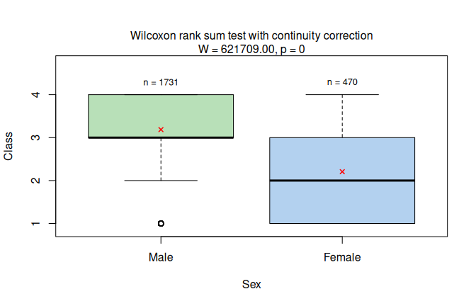

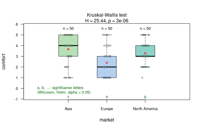
Figure 7.7: Wilcoxon rank-sum test for ordered passenger class by sex in the expanded Titanic data (left) and its multi-group generalisation, the Kruskal-Wallis test for ordered car comfort ratings by market (right). Holm-adjusted pairwise Wilcoxon post-hoc comparisons are shown as significance letters for the Kruskal-Wallis example (\(\alpha = 0.05\)).

7.3 Route 3: Numeric response, numeric predictor

7.3.1 Linear regression

The swiss dataset records standardised fertility and socio-economic indicators for 47 French-speaking Swiss provinces in 1888. We examine how the share of draftees achieving the highest army examination score (Examination) predicts the fertility measure (Fertility), with conf.level = 0.99. The diagnostic panel in Figure 7.8, left, shows that both normality tests pass and the Breusch–Pagan test confirms homoscedasticity, supporting the linear model. The assumption-diagnostic panel is displayed, but its checks do not trigger automatic model replacement. The regression plot shows the fitted line

\[\begin{equation} \hat{y}_i = b_0 + b_1 x_i \tag{7.1} \end{equation}\] with the point estimates \(b_0\) and \(b_1\) for the unknown parameters \(\beta_0\) and \(\beta_1\) of the linear regression model in Eq. (5.1) with one predictor. It is displayed with pointwise confidence and prediction bands at the specified conf.level.

The returned object contains the regression statistics, residual-normality tests, pointwise confidence and prediction bands, and the coefficient of determination \(R^2\) (Eq. (F.1)) as effect size.

linreg_swiss <- visstat(swiss$Examination, swiss$Fertility, conf.level = 0.99)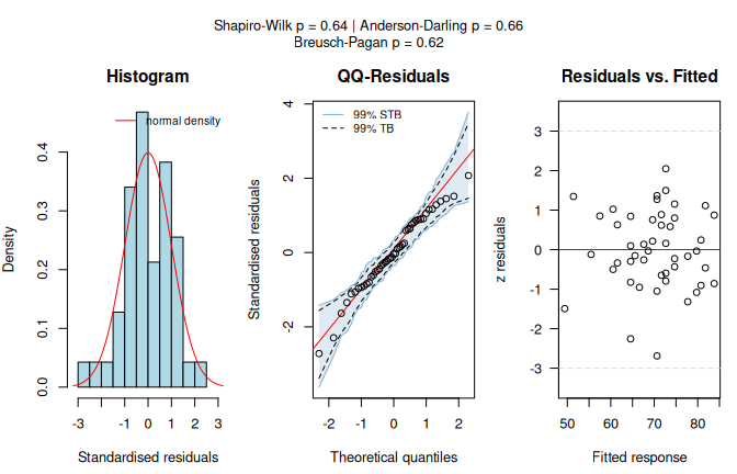

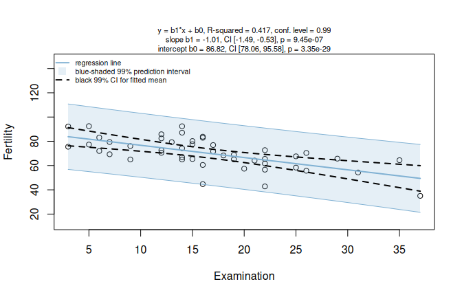
Figure 7.8: Simple linear regression of Fertility on Examination for the swiss dataset (conf.level = 0.99). Assumption diagnostics (Shapiro–Wilk, Anderson–Darling, Breusch–Pagan) and scatter plot with fitted regression line, blue-shaded 99% prediction interval, and black 99% CI for the fitted mean.

The airquality ozone example shows the limits of the automated approach when the default linear model is not an adequate final model. visstat() identifies assumption violations and points to analyses outside the automated decision tree. A default visstat() call for ozone concentration (Ozone) as a function of wind speed (Wind) fits the simple linear model.

ozone_lm <- visstat(airquality$Wind, airquality$Ozone)

## Warning: Statistical assumptions violated:
## Normality of residuals violated (Shapiro-Wilk p = 0.00522 )
## Homoscedasticity violated (Breusch-Pagan p = 0.00595 )
## Analysis proceeded but interpret results cautiously.

## RECOMMENDATION: Consider exploring alternatives outside visstat() such as data transformations,
## generalised linear models, or robust regression. For a non-causal alternative
## consider rerunning with correlation = TRUE.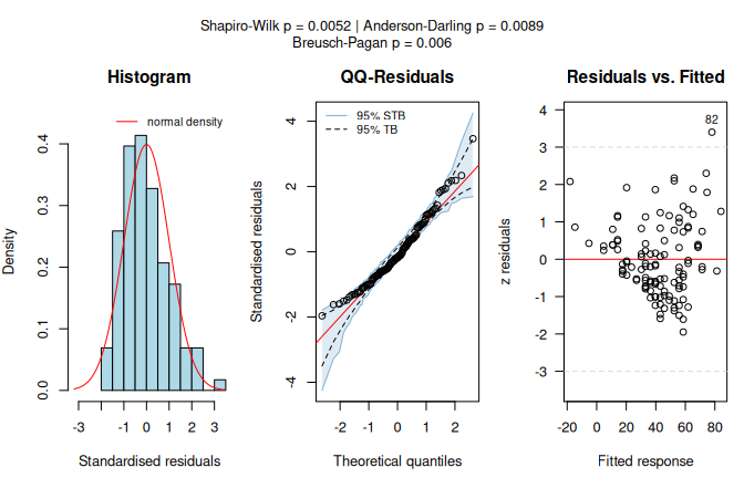

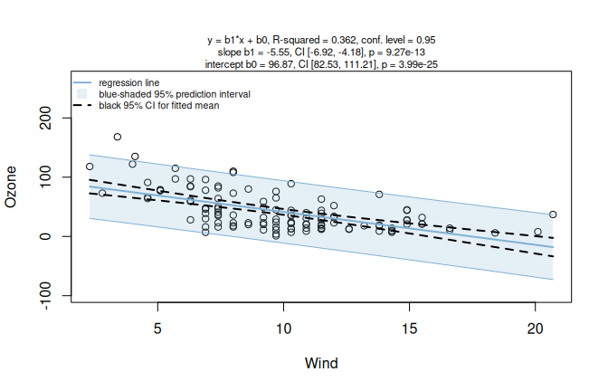
Figure 7.9: Default simple linear regression for Ozone by Wind in the airquality dataset. Assumption diagnostics flag non-normal model residuals and heteroscedasticity before alternative routes are considered.

The diagnostic output flags non-normal model residuals and heteroscedasticity.

In the “Residual vs. fitted” diagnostic panel we observe an increase in spread from left to right, forming a funnel shape that indicates variance increases with fitted values. The optional Spearman analysis for the same dataset is shown in Section 7.5. The following example shows a Gamma generalised linear model outside visstat().

7.3.2 Model exploration outside visstat()

As a model outside of visstat(), we fit a Gamma generalised linear model with log link. The Gamma family is suited here because Ozone is strictly positive and continuous, and its variance grows with the fitted values — the structure detected by the Breusch–Pagan test. The log link guarantees positive fitted values.

# Gamma model with log mapping
model_gamma <- glm(Ozone ~ Wind, data = airquality, family = Gamma(link = "log"))
model_gamma$aic

## [1] 1040.021

#Comparison with AIC of simple linear regression
model_lm <- glm(Ozone ~ Wind, data = airquality)
model_lm$aic

## [1] 1093.187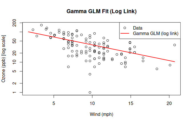

Figure 7.10: Gamma GLM with log link fitted to the airquality dataset Ozone vs. Wind. The red curve shows the fitted Gamma GLM; the y-axis is on a log scale.

For a Gamma generalised linear model with log link, standardised deviance residuals are asymptotically standard normal; we use Shapiro–Wilk and Anderson–Darling as approximate checks of the fitted model:

# Extract standardised deviance residuals
std_dev_res <- rstandard(model_gamma, type = "deviance")
# Validate using the Shapiro-Wilk normality test
shapiro.test(std_dev_res)

## 
##  Shapiro-Wilk normality test
## 
## data:  std_dev_res
## W = 0.99245, p-value = 0.7817

# Validate using the Anderson-Darling normality test
nortest::ad.test(std_dev_res)

## 
##  Anderson-Darling normality test
## 
## data:  std_dev_res
## A = 0.198, p-value = 0.8853

The Gamma model improves the model fit according to the Akaike Information Criterion (Akaike 1974), which decreases from 1093.2 to 1040.0. The increase in the Shapiro–Wilk \(p\)-value from \(p_{SW} = 0.0052\) in the simple linear regression to \(p_{SW} = 0.78\) is more consistent with residual normality. This comparison illustrates how assumption warnings from visstat() can motivate model exploration outside the automated decision tree.

7.4 Route 4: Two unordered factors

The following examples are based on the HairEyeColor contingency table, which is converted to the column-based data frame expected by visstat() using the helper function counts_to_cases().

7.4.1 Pearson’s \(\chi^2\) test

For a contingency table with \(R\) response levels and \(C\) predictor levels, Pearson’s \(\chi^2\) test (Eq. (D.2)) shows a grouped column plot of row percentages with the \(p\)-value in the title, followed by a mosaic plot from vcd (Meyer et al. 2006, 2024). Each tile corresponds to one cell of the contingency table. The tile colour represents the Pearson residual value (Eq. (D.1)) on a blue–red colour scale; the tile size reflects the cell count.

With Eye and Hair from HairEyeColor, all expected cell counts exceed the Cochran thresholds (Cochran 1954), so the \(4 \times 4\) \(\chi^2\) approximation is used.

hair_eye_df <- counts_to_cases(as.data.frame(HairEyeColor))
visstat(hair_eye_df$Eye, hair_eye_df$Hair)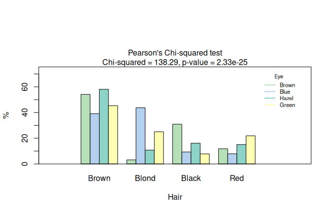

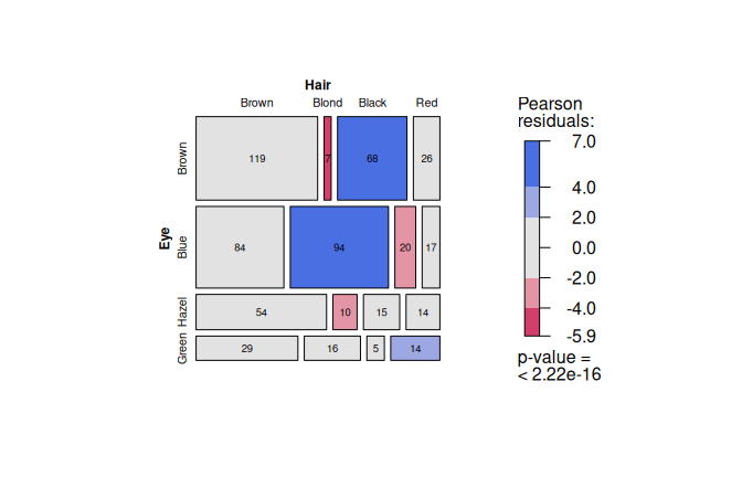
Figure 7.11: Pearson’s \(\chi^2\) test applied to the HairEyeColor dataset. Grouped bar chart of eye colour by hair colour and mosaic plot with tiles coloured by Pearson residuals (blue: over-represented, red: under-represented).

Here, cells for black hair and brown hair, as well as blond hair and blue eyes, show counts above the expectation.

7.4.2 Pearson’s \(\chi^2\) test with Yates’ continuity correction

Restricting HairEyeColor to black or brown hair and brown or blue eyes yields a \(2 \times 2\) table. Cochran’s rule is still satisfied, so visstat() applies Pearson’s \(\chi^2\) test with Yates’ continuity correction. The resulting grouped column plot is shown in Figure 7.12, left.

hair_black_brown_eyes_brown_blue <- HairEyeColor[1:2, 1:2, ]
hair_black_brown_eyes_brown_blue_df <- counts_to_cases(
  as.data.frame(hair_black_brown_eyes_brown_blue))
yates_stats <- visstat(hair_black_brown_eyes_brown_blue_df$Eye,
                       hair_black_brown_eyes_brown_blue_df$Hair)

yates_stats$effect_size

## $name
## [1] "phi"
## 
## $estimate
## [1] 0.1709571
## 
## $effect_size_method
## [1] "Phi coefficient for 2 x 2 contingency table"

The returned effect size is \(\phi = 0.17\), which, using Cohen’s benchmarks for \(2 \times 2\) tables (Cohen 2013, 227), is a small association. The p-value instead is below \(\alpha = 0.05\) (\(p = 0.0035\)) and thus significant. This example underlines the importance of effect sizes: a significant p-value can be accompanied by a small effect size measure.

7.4.3 Fisher’s exact test

Restricting HairEyeColor to male participants with black or brown hair and hazel or green eyes yields a \(2 \times 2\) table where one expected frequency is less than 5, violating Cochran’s rule (Cochran 1954). visstat() therefore applies Fisher’s exact test. The graphical output shows absolute counts with count labels above each bar and the \(p\)-value in the title, so the small cell counts that trigger the exact test remain visible (see Figure 7.12, right).

hair_eye_male <- HairEyeColor[, , 1]
black_brown_hazel_green <- hair_eye_male[1:2, 3:4]
black_brown_hazel_green_df <- counts_to_cases(
  as.data.frame(black_brown_hazel_green))
fisher_stats <- visstat(black_brown_hazel_green_df$Eye,
                        black_brown_hazel_green_df$Hair)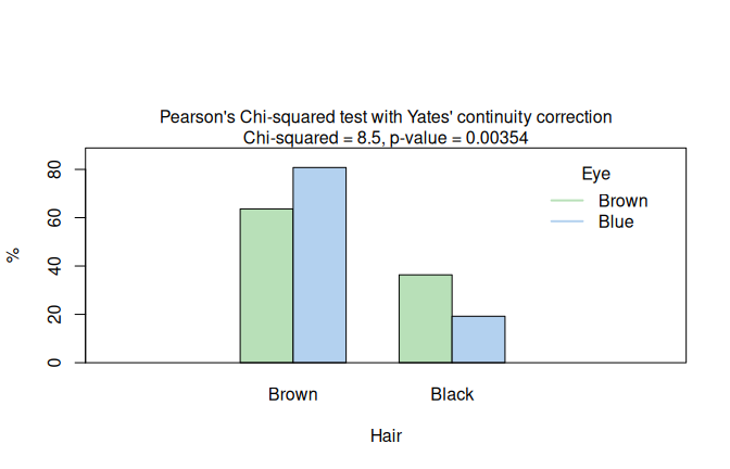

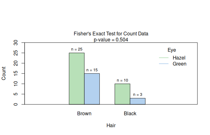
Figure 7.12: Two \(2 \times 2\) categorical routes in HairEyeColor: Yates-corrected Pearson \(\chi^2\) when Cochran’s rule is satisfied (black/brown hair and brown/blue eyes; left), and Fisher’s exact test when expected counts are too small (male participants, black/brown hair, hazel/green eyes; right). The Yates-corrected plot shows row percentages; the Fisher plot shows absolute counts.

7.5 Optional rank-correlation mode

Correlation analysis requires the explicit flag correlation = TRUE.

7.5.1 Kendall rank correlation with correlation = TRUE

A hypothetical survey of 150 secondary-school students records alcohol consumption frequency and academic performance on five-point ordinal scales. A negative monotone association is induced by construction: students who consume alcohol more frequently tend to have lower academic performance. The Kendall result is shown in Figure 7.13, left.

set.seed(42)
n <- 150
xs <- sample(1:5, n, replace = TRUE)
ys <- pmin(5, pmax(1, (6 - xs) + sample(-1:1, n, replace = TRUE)))
likert_alc  <- c("never", "rarely", "sometimes", "often", "always")
likert_perf <- c("poor",  "fair",   "ok",        "good",  "great")
alcohol     <- ordered(likert_alc[xs],  levels = likert_alc)
performance <- ordered(likert_perf[ys], levels = likert_perf)
kendall_result <- visstat(performance, alcohol, correlation = TRUE)
spearman_air <- visstat(airquality$Wind, airquality$Ozone, correlation = TRUE)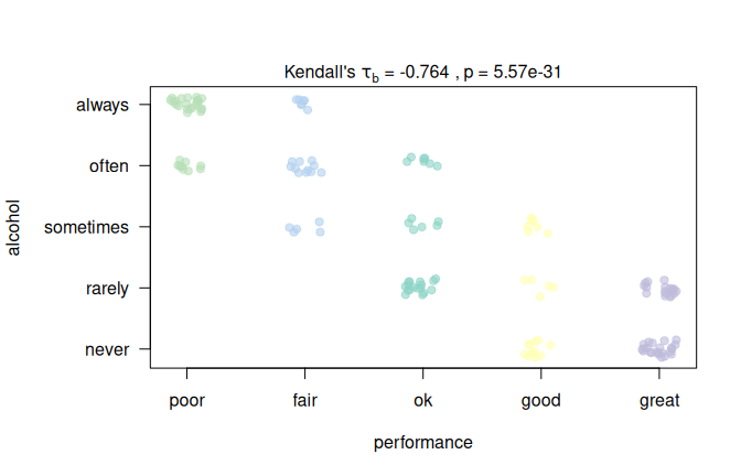

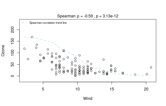
Figure 7.13: Rank-based correlations: Left: Kendall’s \(\tau_b\) for a hypothetical survey (\(n = 150\)): alcohol consumption frequency vs. academic performance. Right: Spearman rank correlation of Wind and Ozone from the airquality dataset (correlation = TRUE; right). Both plots annotate the corresponding effect measure and \(p\)-value.

7.5.2 Spearman rank correlation with correlation = TRUE

For the ozone example introduced in Section 7.3.1, staying within visstat() with the flag correlation = TRUE gives the Spearman analysis shown in Figure 7.13, right.

8 Discussion

For every chosen test, visStatistics provides both a visualisation and a full report covering the test itself, and, where applicable, its assumption checks and post-hoc comparisons. The report is complemented by each test’s effect size (Table F.1): A sufficiently large sample makes even a negligible difference significant, so the p-value must be read alongside the magnitude of the effect (Levine and Hullett 2002; Cohen 2013, 10). The “right” test is thus per se not the one with the smallest p-value, but one whose assumptions hold, and whose effect is large enough to matter.

For tests of central tendency, p-values from assumption tests of normality and homoscedasticity are used as routing criteria, subject to the large sample-size safeguards discussed below for normality testing. However, no single assumption test maintains optimal Type I error rates and statistical power across all distributions (Olejnik and Algina 1987) and sample sizes, and p-values obtained from these tests may be unreliable if their assumptions are violated.

Assessing assumptions solely through p-values can lead to both type I errors (false positives) and type II errors (false negatives). In large samples, even minor, random deviations from the null hypothesis can result in statistically significant p-values, leading to type I errors. Conversely, in small samples, substantial violations of the assumption may not reach statistical significance, resulting in type II errors (Kozak and Piepho 2018). Thus, the robustness of statistical tests depends on both the sample size and the shape of the underlying distribution.

In tests comparing group means, the Central Limit Theorem (CLT) allows us to bypass the formal assessment of the residual normality in large samples:
By the CLT, the sampling distribution of the group means approaches normality as the group sizes grow, regardless of the shape of the underlying distribution. For finite group sizes this holds only approximately, but it implies that in large enough samples a rejected residual-normality test no longer threatens the validity of the mean-based test. This raises the practical question of what should count as a “large enough” sample. The answer depends on the shape of the underlying distribution, especially skewness and tail weight (Lumley et al. 2002).

visstat() tests the residual normality before testing homoscedasticity, so the justification of the minimum group size to bypass the residual normality testing must hold for both mean-based families it might reach: the homoscedastic comparison—Student’s t-test, generalised to Fisher’s one-way ANOVA—and the heteroscedastic comparison—Welch’s t-test, generalised to Welch’s one-way ANOVA. Monte Carlo studies of robustness to non-normality (Blanca et al. 2017; Fagerland 2012; Delacre et al. 2019) examine both mean-based families against a common criterion: under the null hypothesis of equal population means, and at a significance level of \(\alpha = 5\%\), the empirical Type I error rate must stay within Bradley’s liberal robustness bounds of \([2.5\%, 7.5\%]\) (Bradley 1978).

In the context of homoscedastic comparison, Blanca et al. (Blanca et al. 2017) demonstrated in a three-group design that the empirical Type I error of Fisher’s one-way ANOVA — whose two-group special case is Student’s t-test — remained within Bradley’s bounds across skewness values up to 2 and kurtosis values up to 6, at group sizes ranging from 5 to 100. For the Student’s t-test, the margin is wider, with a Type I error rate between 4% and 5% for sample sizes of 10 or more, as long as skewness is up to 4 and there are moderate differences in spread (Fagerland 2012).

In the context of heteroscedastic comparison, Delacre et al. (Delacre et al. 2019) established that the empirical Type I error of Welch’s one-way ANOVA – whose two-group special case is Welch’s t-test – remained within Bradley’s bounds at approximately 50 observations per group for up to four groups. With more than four groups, 50 observations still suffice for skewness up to 2, for higher skewness roughly 100 per group are required.

Summing up, the Central Limit Theorem and these simulation studies indicate that a minimum group size of 50 is a conservative threshold for skewness up to about 2. Above this size, normality tests of residuals do not steer automated routing in the decision logic of visstat(), which defaults to mean-based testing independent of the shape of the sample distribution.

Without this bypass, the Shapiro–Wilk test would reject residual normality for almost any skewed sample at these sizes and reroute the comparison to a rank-based test. Such a switch is not more valid, because the Central Limit Theorem has already secured the mean-based comparison; it only answers a different question, about medians rather than means.

Drop the n>50 bypass; SW routes at every n. No size threshold to justify — and none is defensible, since the “large enough” cut-off depends on skew and group count. Large n: SW over-rejects skewed data → routes to rank; passes near-normal data → mean. The over-rejection is not a flaw — it sends skewed samples to the rank test, the more powerful and more appropriate question there. Forcing means above 50 was never justified. Small n: SW is underpowered → usually passes → mean test; only strong skew is caught → rank. For skew<1 this is correct (mean ≈ median, t and rank essentially equal power); missed mild skew costs little (Bridge). Cost: the conditional pretest inflates Type I only slightly (~0.05–0.07, within Bradley).

Large n: SW over-rejects  mildly skewed data → routes to rank; passes near-normal data → mean. The over-rejection is  a flaw — it sends nearly normal  samples to the rank test, minimal loss of power, change of null

visstat routes on a residual-normality p-value, a sample-size-dependent proxy for the shape (skewness, tail weight) that actually governs whether the mean is a faithful estimand. A shape-selector would be more principled (Hall and Padmanabhan 1997), but sample shape is poorly estimated in the small samples where the choice matters and admits no non-arbitrary threshold. SW is used because it is the transparent diagnostic already displayed, not because it is the optimal selection statistic.

For smaller group-specific sample sizes, a Shapiro–Wilk test is used to route between mean-based and rank-based methods, as simulation studies suggest that it has the highest power among normality tests in small to moderate (\(n = 10\) to 100) sample sizes (Razali and Wah 2011).

Because the Shapiro–Wilk test’s power against non-normality is driven primarily by asymmetry at small-to-moderate sample sizes (Razali and Wah 2011), a rejected residual-normality test acts here as a practical proxy for the skewness that determines whether the mean is a faithful summary (Eq. (A.1); supplementary simulation).

Shapiro–Wilk serves as a proxy for skewness, the feature deciding whether the mean is a faithful summary: its power against non-normality is driven primarily by asymmetry at small-to-moderate n n (Razali and Wah 2011). It is a normality verdict, not a skewness magnitude — a proxy, not a skewness test. Pre-testing distorts the error rate of any single conditional arm, yet the residual-normality-gated procedure holds the nominal level as a whole (Rochon et al. 2012), reproduced across input distributions from skew 0 to 6 (supplementary); the worst that can be said of the gate is that it is unnecessary, not that it inflates Type I.

Shapiro–Wilk acts as a skewness proxy in the routing: its power against non-normality is driven primarily by asymmetry (Razali and Wah 2011), so the gate effectively responds to skew. In large samples it rejects even mild skew and routes such data to the rank branch, at negligible cost — rank tests retain ~95% efficiency under normality and gain power under skew (Jr 2026; Bridge and Sawilowsky 1999) (supplementary)

Shapiro–Wilk acts as a skewness-sensitive gate: it has high power against skewed alternatives at small-to-moderate N (Razali and Wah 2011). For large N it rejects even mild skew and routes such data to the rank branch, at negligible cost — rank tests retain ~95% efficiency under normality and gain power under skew (Jr 2026; Bridge and Sawilowsky 1999) (supplementary).

Low skew, any N: SW usually stays parametric; even when it does route to rank, mean≈median so the two p-values agree in direction despite the different H₀. No practical harm. ✓ (your point 2) High skew, very small per-group N (~10): SW misses the skew and wrongly stays parametric — the one genuinely wrong outcome. ✓ It self-corrects fast: by ~20/group the skew is caught and routing is correct. At trivially small data (≈5/group) inference is meaningless regardless — so the residual failure sits in a region where no method helps. ✓

Shapiro–Wilk acts as a skewness-sensitive gate: it has high power against skewed alternatives at small-to-moderate N N (Razali and Wah 2011). For large N N it rejects even mild skew and routes such data to the rank branch; the cost of this is not power — rank tests retain ~95% efficiency under normality (Jr 2026; Bridge and Sawilowsky 1999) — but the change of research question from means to stochastic ordering.

A maximally powerful test is useless if it answers the wrong question; lacking the user’s research question, visstat() lets the residual-normality test guess the estimand from shape — transparent and overridable.

Although the Shapiro–Wilk test is an omnibus normality statistic — sensitive to both skewness and excess kurtosis, and by construction unable to indicate which — its power is dominated by asymmetry (Razali and Wah 2011); it therefore acts in practice as a skewness gate, and visstat() uses its rejection of residual normality to route skewed data to rank-based comparison by default.

• What the gate actually is. The Shapiro–Wilk statistic is an omnibus normality test, sensitive to both skewness (\(\sqrt{b_1}\)) and kurtosis (\(b_2\)) though built from neither (D’Agostino and Pearson 1973); because its power is dominated by skewness (Razali and Wah 2011), it functions in practice as a skewness detector — the feature that governs whether a mean is a meaningful summary of each group.

• Why the \(n > 50\) bypass is removed. Since the Shapiro–Wilk test already routes by shape at every \(N\), a sample-size threshold is redundant, and its “large enough” cutoff is itself shape-dependent and therefore arbitrary (Lumley et al. 2002); visstat() thus lets the residual-normality test steer the route at all \(N\) rather than forcing a mean-based test above a fixed size.

• How it behaves, and the real cost. At large \(N\) the gate routes even mildly skewed data to the rank branch; at small \(N\) it is underpowered and keeps moderate skew on the mean route. The cost of this is not power — rank tests retain about 95% efficiency under normality and gain under skew (Jr 2026; Bridge and Sawilowsky 1999) — but a change in the hypothesis tested, from equality of means to stochastic ordering (Fagerland and Sandvik 2009), which visstat() makes explicit by naming the selected test.

• Validity of the whole procedure, and honest scope. Although pre-testing distorts the conditional error of a single arm, the residual-normality-gated procedure holds the nominal level as a whole (Rochon et al. 2012), reproduced in our simulations across distributions from skew 0 to 6 (supplementary); the Shapiro–Wilk test is used because it is the transparent diagnostic already displayed and a serviceable estimand heuristic for an automated tool that is not told the research question — not because it is the optimal selection statistic, a role a shape selector would fill more naturally (Hall and Padmanabhan 1997). against the competitors Recommendations to default unconditionally to Welch’s mean-based test (Delacre et al. 2019; Zimmerman 2004) or to rank-based methods (Jr 2026; Franc 2025) each fix the estimand in advance — means or stochastic ordering — without flagging that the two answer different questions (Fagerland and Sandvik 2009). visstat() instead selects between mean- and rank-based tests of central tendency from the residual diagnostics and reports which was used, leaving the choice visible rather than silently fixed. why both branches Retaining the mean-based branch is not merely conventional. Under normality the general-linear-model tests are uniformly most powerful unbiased (Bridge and Sawilowsky 1999), and they yield effect estimates and confidence intervals on the data’s own scale, together with the regression and ANOVA decomposition that the rank route does not provide (Jr 2026). The rank tests buy robustness and efficiency under skew but give a \(p\)-value without a natural-scale effect or interval. visstat() therefore keeps both and selects between them, rather than discarding the mean framework’s interpretability or the rank framework’s robustness a priori.

*** Codex**Route 1 defaults to parametric tests of central tendency. The assumption tests check whether this default is defensible for the fitted group model, not whether the user’s scientific target is correct. The first check is the shape of the model residuals: after group means have been fitted, the remaining within-group deviations should be compatible with the parametric model. If this residual shape is clearly non-normal, visstat() falls back to ranks.

The weak case is mild skewness of the within-group distributions. In that case, residuals can fail Shapiro-Wilk although the group mean still lies close to the median and still describes the bulk of the observations. Then the rank fallback is conservative, not automatically better

A type I error in a test of homoscedasticity is of no real consequence: it merely routes homoscedastic data to Welch’s t-test or Welch’s one-way ANOVA, which loose only negligible power to Student’ t-test or Fisher Oneway Anova, when variances are in fact equal (Rasch et al. 2011; Delacre et al. 2019).

In the case of balanced designs and equal variances, Welch’s t-test is even algebraically equivalent to Student’s t-test (Eqs. (B.4) and (B.1)) and Welch’s one-way ANOVA converges asymptotically to the Fisher One Way Anova (Eqs. (B.6) and (B.2)). Some authors therefore recommend the Welch tests as the default (Rasch et al. 2011; Delacre et al. 2019).

If the assumptions of parametric tests are violated, visstat() automatically falls back to non-parametric tests. In the regression branch, violated assumptions are solely flagged, and the package offers Spearman rank correlation as a non-causal alternative to linear regression. Further alternative methods such as data transformation, generalised linear models, or robust regression are not implemented: each requires user judgment – about the transformation family, the link function, or the estimator – that cannot be automated without substantially expanding the decision tree and increasing the risk of Type I error inflation.

Assumption tests provide no information on the nature of deviations from the expected distribution (Shatz 2024) and cannot replace visual inspection of the diagnostic plots generated by visstat(), which may indicate cases where the automatic test choice should be overridden.

9 Limitations

The design of visStatistics prioritises transparent, reproducible routing for common two-variable analyses (Strasak et al. 2007; Sato et al. 2017; Chicco et al. 2025) over broad model coverage. This scope keeps the decision tree inspectable and the graphical output consistent, but it also leaves several modelling choices (e.g. paired tests, interaction terms, multiple linear regression) outside the automated workflow.

While one of R’s greatest strengths is the sheer volume of statistical methods available, incorporating a wider array of methods would require additional preliminary assumption checks, which in turn would exacerbate the risk of overall Type I error inflation. Furthermore, expanding the pipeline would result in a highly complex decision tree, rendering the underlying statistical logic increasingly opaque to the user.

Bootstrapping represents an alternative to assumption-guided routing. As implemented for example in the R package boot (Canty and Ripley 2025; Davison and Hinkley 1997), it can provide confidence intervals for a wide range of statistics. However, bootstrapping often requires thousands of resamples and may perform poorly with very small sample sizes. This runs counter to the purpose of the visStatistics package, which is designed to offer a rapid overview of the data, laying the groundwork for deeper analysis in subsequent steps.

At the graphical level, the design is also kept deliberately low-dependency. The package uses mostly R graphics, keeping the transitive dependency footprint minimal. For more polished, annotated plots of chosen statistical tests, we refer to packages such as ggstatsplot (Patil 2021) or ggpubr (Kassambara 2026).

Taken together, these scope decisions define visStatistics as a rapid, inspectable first-line workflow for routine two-variable inference rather than a replacement for model-specific statistical analysis.

10 Conclusion

Many routine statistical analyses reduce to a relatively small number of tests implemented in visStatistics. Among those, parametric tests such as t-tests, analysis of variance, or simple linear regression belong to the family of general linear models, whose assumptions are frequently not tested at all or not tested properly (Hoekstra et al. 2012; Ernst and Albers 2017; Jones et al. 2025; Kéry and Hatfield 2003).

visStatistics addresses this gap: Its selection of tests of central tendencies takes p-values of assumption tests of the model residuals of a fitted linear model into account.

The package addresses the inherent shortcomings of test selection based on p-values (Lumley et al. 2002; Fagerland 2012; Kozak and Piepho 2018; Shatz 2024) by supplementing the output with diagnostic plots of the assumption tests of the selected test. It’s design is therefore a combination of both “assumption checking” (Shatz 2024) by visualisation and “assumption testing” by p-values.

Its value is not that it removes the user’s statistical judgment, but that it exposes the assumptions, effect sizes, and plots that should inform that judgment.

Appendix

A Assumption tests

A.1 Normality tests

A.1.1 Shapiro–Wilk test shapiro.test()

The Shapiro–Wilk test evaluates whether a sample \(x_1,\ldots,x_n\) comes from a normal distribution. Let \(x_{(1)}\le \cdots \le x_{(n)}\) be its order statistics. Introduce a reference sample \(Z_1,\ldots,Z_n\) of independent standard normal random variables, i.e. \(Z_i \sim N(0,1)\) for all \(i\), and let \(Z_{(1)}\le \cdots \le Z_{(n)}\) be their order statistics used to construct the Shapiro–Wilk weights.

Let \(m_i = \operatorname{E}(Z_{(i)})\) and \(v_{ij} = \operatorname{Cov}(Z_{(i)}, Z_{(j)})\) for \(i,j = 1,\ldots,n\). Define \(\mathbf{m} = (m_1,\ldots,m_n)^\top\) and \(V = (v_{ij})_{i,j=1}^n\).

The vector \(\mathbf{m}\) contains the expected standard-normal order statistics, and \(V\) is their covariance matrix. Let \(\mathbf{a}=(a_1,\ldots,a_n)^\top\) be the resulting vector of normalised weights for the ordered observed sample values

\[\mathbf{a} =\frac{V^{-1}\mathbf{m}} {\sqrt{\left(\mathbf{m}^\top V^{-1}V^{-1}\mathbf{m}\right)}}.\] Then the Shapiro–Wilk statistic (Shapiro and Wilk 1965) is

\[\begin{equation} W=\frac{\left(\sum_{i=1}^{n} a_i x_{(i)}\right)^2} {\sum_{i=1}^{n} (x_i-\bar{x})^2} \tag{A.1} \end{equation}\]

\(W\) takes values in \((0, 1]\); values close to 1 indicate normality.

A.1.2 Anderson–Darling test ad.test()

Let \(z_i = (x_{(i)} - \bar{x})/s,\; i=1,2,\ldots,n\) be the standardised order statistics of \(x_i\), where \(s\) is the sample standard deviation, and let \(\Phi\) denote the standard normal cumulative distribution function. The test statistic is

\[\begin{equation} A^2 = -n - \frac{1}{n}\sum_{i=1}^{n}(2i-1) \left[\ln\Phi(z_i) + \ln\!\left(1 - \Phi(z_{n+1-i})\right)\right] \tag{A.2} \end{equation}\]

The implementation uses ad.test() from nortest (Gross and Ligges 2015).

A.2 Homoscedasticity tests

A.2.1 The mean-centred Levene test levene.test()

The package implementation uses Levene’s original mean-centred proposal (Levene 1960).

The Levene test statistic is the one-way ANOVA \(F\) statistic, computed on the absolute residuals \(|e_{ij}|\) in place of the responses \(x_{ij}\); the corresponding Fisher ANOVA formula is given in Eq. (B.2):

\[\begin{equation} F_L = \frac{\displaystyle\sum_{i=1}^{k} n_i (\overline{|e|}_i - \overline{|e|})^2\;/\;(k-1)} {\displaystyle\sum_{i=1}^{k}\sum_{j=1}^{n_i}(|e_{ij}| - \overline{|e|}_i)^2\;/\;(N-k)}, \tag{A.3} \end{equation}\]

where \(\overline{|e|}_i\) is the within-group mean of the absolute residuals and \(\overline{|e|}\) is their overall mean.

A.2.2 Bartlett’s test bartlett.test()

Bartlett’s test statistic (Bartlett 1937) is

\[\begin{equation} K^2 = \frac{(N-k)\ln s_p^2 - \displaystyle\sum_{i=1}^k (n_i-1)\ln s_i^2} {1 + \dfrac{1}{3(k-1)}\!\left(\displaystyle\sum_{i=1}^k \frac{1}{n_i-1} - \frac{1}{N-k}\right)}, \tag{A.4} \end{equation}\]

where \(k\) is the number of groups, \(N = \sum_{i=1}^k n_i\) is the total sample size, \(n_i\) is the sample size of group \(i\), \(s_i^2\) is the sample variance of group \(i\), and \(s_p^2\) is the pooled variance

\[s_p^2 = \frac{1}{N-k}\sum_{i=1}^k (n_i-1)\,s_i^2.\]

Under the null hypothesis the statistic approximately follows \(\chi^2(k-1)\).

A.2.3 Breusch–Pagan test bp.test()

For simple linear regression, group-based variance tests are not applicable. The package implementation bp.test() performs the Koenker variant (Koenker 1981) of the Breusch–Pagan test (Breusch and Pagan 1979), which tests whether the \(N\) squared residuals \(e_i^2\) vary systematically with the fitted values from the regression model \(\hat{y}_i\).

The Breusch–Pagan statistic is defined as:

\[\begin{equation} BP = N R^2_\text{aux} \tag{A.5}, \end{equation}\]

where \(R^2_\text{aux}\) denotes the coefficient of determination from regressing \(e_i^2\) on \(\hat{y}_i\):

\[R^2_\text{aux} = 1 - \frac{\sum_{i=1}^{N} (e_i^2 - \widehat{e_i^2})^2} {\sum_{i=1}^{N} (e_i^2 - \overline{e^2})^2}.\]

Here \(\widehat{e_i^2}\) are the fitted values from this auxiliary regression and \(\overline{e^2}\) is the mean of the squared residuals.

Under the null hypothesis of homoscedasticity, \(BP\) is compared asymptotically to a \(\chi^2(k-1)\) distribution.

B Parametric tests

In the numeric-response, categorical-predictor branch (Route 1), parametric tests are selected when residual normality is not rejected, or when all group-specific sample sizes are greater than 50. The Levene variance gate then separates equal-variance tests from Welch-type tests.

B.1 Student’s t-test and Fisher’s one-way ANOVA

B.1.1 Student’s t-test t.test(..., var.equal = TRUE)

Student’s t-test tests the null hypothesis that the population means of two unpaired groups are equal. The test statistic for Student’s t-test (t.test(..., var.equal = TRUE)) is

\[\begin{equation} t = \frac{\bar{x}_1 - \bar{x}_2} {s_p \sqrt{\dfrac{1}{n_1} + \dfrac{1}{n_2}}}, \tag{B.1} \end{equation}\]

where \(\bar{x}_1\) and \(\bar{x}_2\) are the sample means, \(n_1\) and \(n_2\) the sample sizes, and \(s_p\) the pooled standard deviation

\[s_p = \sqrt{\frac{(n_1-1)s_1^2 + (n_2-1)s_2^2}{n_1+n_2-2}},\]

with \(s_1^2\) and \(s_2^2\) the sample variances. The statistic follows a \(t\)-distribution with \(\nu = n_1 + n_2 - 2\) degrees of freedom.

B.1.2 Fisher’s one-way ANOVA aov()

Fisher’s one-way ANOVA generalises the comparison to more than two groups and tests the null hypothesis that the population means of \(k\) groups are equal. Fisher’s ANOVA test statistic is

\[\begin{equation} \begin{aligned} F &= \frac{MS_\text{between}}{MS_\text{within}} = \frac{SS_\text{between}/(k-1)}{SS_\text{within}/(N-k)} = \frac{\displaystyle\sum_{i=1}^{k} n_i (\bar{x}_i - \bar{x})^2\;/\;(k-1)} {\displaystyle\sum_{i=1}^{k}\sum_{j=1}^{n_i} (x_{ij}-\bar{x}_i)^2\;/\;(N-k)} \end{aligned}, \tag{B.2} \end{equation}\]

where \(MS_\text{between}\) and \(MS_\text{within}\) are the between-group and within-group mean squares, \(SS_\text{between}\) and \(SS_\text{within}\) are the corresponding sums of squares, \(k\) is the number of groups, \(N = \sum_{i=1}^k n_i\) is the total sample size, \(\bar{x}_i\) is the mean of group \(i\), \(\bar{x}\) is the overall mean, and \(x_{ij}\) is observation \(j\) in group \(i\).

From Eq. (B.2) follows that in the two-sample case (\(k=2\)), the squared test statistic of Student’s t-test equals the Fisher ANOVA test statistic, \(t^2 = F\), resulting in identical \(p\)-values for t.test(var.equal = TRUE) and aov().

Under \(H_0: \mu_1 = \cdots = \mu_k\), the statistic follows \(F(k-1, N-k)\).

B.1.2.1 Post-hoc comparison

visstat() follows aov() with Tukey’s Honest Significant Differences procedure TukeyHSD() (Tukey 1949). The procedure is designed for pairwise mean comparisons following ANOVA.

TukeyHSD() returns adjusted p-values and confidence intervals for all pairwise differences between factor-level means. For two groups \(i\) and \(j\), let \(d_{ij} = \bar{x}_i - \bar{x}_j\). The studentised range statistic is

\[\begin{equation} q_{ij} = \frac{|d_{ij}|} {\sqrt{\dfrac{MS_\text{within}}{2} \left(\dfrac{1}{n_i} + \dfrac{1}{n_j}\right)}}, \tag{B.3} \end{equation}\]

where \(MS_\text{within}\) is defined in Eq. (B.2). Adjusted p-values are computed from the studentised range distribution with \(k\) groups and \(N-k\) residual degrees of freedom.

B.2 Welch’s t-test and Welch’s heteroscedastic ANOVA

Welch’s heteroscedastic ANOVA generalises the unequal-variance mean comparison to more than two groups.

B.2.1 Welch’s t-test t.test()

Welch’s t-test (t.test(..., var.equal = FALSE)) compares the means of two independent groups when homogeneous variances cannot be assumed. Its statistic is

\[\begin{equation} t = \frac{\bar{x}_1 - \bar{x}_2} {\sqrt{s_1^2/n_1 + s_2^2/n_2}} \tag{B.4} \end{equation}\]

with degrees of freedom approximated by the Welch–Satterthwaite equation (Welch 1947; Satterthwaite 1946):

\[\begin{equation} \nu \approx \frac{\left(\dfrac{s_1^2}{n_1} + \dfrac{s_2^2}{n_2}\right)^2} {\dfrac{(s_1^2/n_1)^2}{n_1-1} + \dfrac{(s_2^2/n_2)^2}{n_2-1}}. \tag{B.5} \end{equation}\]

B.2.2 Welch’s heteroscedastic ANOVA oneway.test()

Welch’s heteroscedastic ANOVA (oneway.test()) generalises Welch’s t-test to more than two groups by down-weighting groups with large variance. It compares group means using weights based on sample sizes and variances when homogeneous variances cannot be assumed. Its test statistic is

\[\begin{equation} F_W = \frac{\displaystyle\sum_{i=1}^{k} w_i (\bar{x}_i - \bar{x}_w)^2\;/\;(k-1)} {1 + \dfrac{2(k-2)}{k^2-1} \displaystyle\sum_{i=1}^{k} \dfrac{(1-w_i/w)^2}{n_i-1}}, \tag{B.6} \end{equation}\]

where \(w_i = n_i/s_i^2\) are the inverse-variance weights, \(w = \sum_{i=1}^{k} w_i\), and \(\bar{x}_w = \sum_{i=1}^{k} w_i \bar{x}_i / w\) is the weighted grand mean. The numerator degree of freedom is \(k-1\); the denominator degree of freedom is the Satterthwaite-type approximation returned by oneway.test().

B.2.2.1 Post-hoc comparison games.howell()

Post-hoc comparisons use the package implementation games.howell() (Games and Howell 1976). The Games–Howell procedure is used for pairwise mean comparisons under unequal variances and unequal sample sizes. For each pairwise comparison, the two groups are denoted as 1 and 2. The test statistic is

\[\begin{equation} t = \frac{d}{SE}, \tag{B.7} \end{equation}\]

where \(d = \bar{x}_1 - \bar{x}_2\) is the mean difference and \(SE = \sqrt{s_1^2/n_1 + s_2^2/n_2}\) its standard error.

Eq. (B.7) is evaluated against a \(t\) distribution with \(\nu\) degrees of freedom from the Welch–Satterthwaite approximation in Eq. (B.5). The resulting two-sided \(p\)-values are adjusted with Holm’s method (Holm 1979).

Welch’s methods outperform their classical counterparts when variances differ (Moser and Stevens 1992; Fagerland and Sandvik 2009; Delacre et al. 2017).

B.2.2.2 Welch’s method in the case of equal variances

When variances are equal, Welch’s methods lose only negligible power relative to their classical counterparts (Moser and Stevens 1992; Delacre et al. 2017).

Welch’s method in the case of equal variances and balanced designs

B.2.2.2.1 Two- group comparison

If variances are equal and the groups are balanced (the same number in each group), the Welch method’s reduce in the case of two -group comparison algebraically to Student’s t-test (equivalent to Fisher - Anova for two groups):

When \(s_1^2 = s_2^2 = s^2\) and \(n_1 = n_2 = n\), the pooled variance entering Eq. (B.1) becomes \[\begin{equation} s_p^2 = \frac{(n-1)s^2 + (n-1)s^2}{2n-2} = s^2, \tag{B.8} \end{equation}\] so the Welch denominator in Eq. (B.4), \(\sqrt{s^2/n + s^2/n} = s\sqrt{2/n}\), equals the Student denominator \(s_p\sqrt{1/n + 1/n} = s\sqrt{2/n}\), and the Welch–Satterthwaite degrees of freedom in Eq. (B.5) reduce to \[\begin{equation} \nu = \frac{\left(2s^2/n\right)^2} {\dfrac{(s^2/n)^2}{n-1} + \dfrac{(s^2/n)^2}{n-1}} = \frac{4s^4/n^2}{2s^4/[n^2(n-1)]} = 2(n-1) = 2n-2. \tag{B.9} \end{equation}\] Welch’s t-test then coincides with Student’s t-test on \(2n-2\) degrees of freedom.

B.2.2.3 More then two groups comparisons

This exact equivalence does not extend beyond two groups: even under equal variances and equal group sizes, the Welch statistic \(F_W\) in Eq. (B.6) is not algebraically identical to the classical \(F\) in Eq. (B.2) for \(k>2\) ; it nevertheless converges to it as \(n\) increases: Under equal variances and equal group sizes, \(s_1^2 = \cdots = s_k^2 = s^2\) and \(n_1 = \cdots = n_k = n\). Hence \(w_i = n/s^2\), \(w = kn/s^2\), \(w_i/w = 1/k\), and \(\bar{x}_w = \bar{x}\). The numerator of Eq. (B.6) then reduces to \[\begin{equation} \frac{\sum_{i=1}^{k} w_i(\bar{x}_i-\bar{x}_w)^2}{k-1} = \frac{1}{s^2} \frac{\sum_{i=1}^{k} n(\bar{x}_i-\bar{x})^2}{k-1} = \frac{MS_\text{between}}{s^2}. \tag{B.10} \end{equation}\]

Because \(MS_\text{within}=s^2\) under the same assumptions, this is the numerator of the classical statistic \(F=MS_\text{between}/MS_\text{within}\). The remaining denominator correction in Eq. (B.6) becomes

\[\begin{equation} 1+ \frac{2(k-2)(k-1)}{k(k+1)(n-1)}. \tag{B.11} \end{equation}\]

Thus

\[\begin{equation} F_W = \frac{F} {1+\dfrac{2(k-2)(k-1)}{k(k+1)(n-1)}}. \tag{B.12} \end{equation}\]

For \(k=2\), the correction term is zero, so Welch’s ANOVA form gives the same statistic as Fisher’s ANOVA Eq. (B.2).

For the four-group case used in the examples, \(k=4\) and therefore

\[\begin{equation} F_W = \frac{F}{1+\dfrac{3}{5(n-1)}}. \tag{B.13} \end{equation}\]

Equivalently, \(F/F_W = 1 + 3/[5(n-1)]\). The relative excess \(F/F_W - 1\) is therefore \(O(n^{-1})\) and, in this four-group example, already below \(1\%\) for \(n > 61\).

C Non-parametric tests

In the numeric-response, categorical-predictor branch, non-parametric tests are selected when residual normality is rejected. They are also used for an ordered response with a categorical predictor.

C.1 Wilcoxon rank-sum test and Kruskal–Wallis test

The Wilcoxon rank-sum test is a two-group rank-based location test; Kruskal–Wallis generalises this location comparison to more than two groups.

C.1.1 Wilcoxon rank-sum test wilcox.test()

The two-sample Wilcoxon rank-sum test, also known as the Mann–Whitney test, tests for a difference in location between two independent distributions.

To compare the two groups on one common rank scale, all observations are pooled before ranking. For two independent groups with sample sizes \(n_1\) and \(n_2\), all \(N = n_1 + n_2\) observations are assigned ranks \(1\) to \(N\). Let \(W_1 = \sum_{i=1}^{n_1} R(x_{1,i})\) denote the rank sum of the first group, where \(R(x_{1,i})\) is the rank of observation \(x_{1,i}\) in the pooled sample. The test statistic returned by wilcox.test() is the Mann–Whitney \(U\) statistic (Mann and Whitney 1947) of the first group:

\[\begin{equation} W = U_1 = W_1 - \frac{n_1(n_1+1)}{2} \tag{C.1} \end{equation}\]

An exact \(p\)-value is computed when both groups contain fewer than 50 observations and the data contain no ties; otherwise a normal approximation with continuity correction is used.

C.1.2 Kruskal–Wallis test kruskal.test()

The Kruskal–Wallis test compares group distributions based on ranked values and tests the null hypothesis that the groups come from the same population, specifically that the distributions have the same location (Kruskal and Wallis 1952). If the group distributions are sufficiently similar in shape and scale, the test can be interpreted as testing equality of medians across groups (Hollander et al. 2014).

\[\begin{equation} H = \frac{12}{N(N+1)} \sum_{i=1}^{k} n_i \left(\bar{R}_i - \bar{R}\right)^2, \tag{C.2} \end{equation}\]

where \(n_i\) is the sample size of group \(i\), \(k\) is the number of groups, \(\bar{R}_i\) is the average rank of group \(i\), \(N\) is the total sample size, and \(\bar{R} = (N+1)/2\) is the expected average rank under the null hypothesis. The statistic approximately follows \(\chi^2(k-1)\).

C.1.2.1 Post-hoc comparison pairwise.wilcox.test()

pairwise.wilcox.test() compares each pair of factor levels via the Wilcoxon rank-sum test on ranks rather than means. The resulting p-values are adjusted for multiplicity using Holm’s step-down method (Holm 1979).

D Tests for comparing proportions

For two unordered factors (route 4), visstat() tests the null hypothesis that the variables are independent using Pearson’s \(\chi^2\) test or Fisher’s exact test, depending on expected cell counts following Cochran’s rule (Cochran 1954).

D.1 Pearson’s \(\chi^2\) test chisq.test()

Pearson’s \(\chi^2\) test evaluates the null hypothesis that two categorical variables are independent.

Let \(O_{ij}\) and \(E_{ij}\) denote the observed and expected frequencies in row \(i\) and column \(j\) of an \(R \times C\) contingency table, where rows index the \(R\) levels of the response \(y\) and columns the \(C\) levels of the predictor \(x\). The Pearson residual for cell \((i,j)\) is \[\begin{equation} r_{ij} = \frac{O_{ij} - E_{ij}}{\sqrt{E_{ij}}}, \quad i = 1,\ldots,R,\quad j = 1,\ldots,C. \tag{D.1} \end{equation}\] The test statistic of Pearson’s \(\chi^2\) test is

\[\begin{equation} \chi^2 = \sum_{i=1}^{R}\sum_{j=1}^{C} r_{ij}^2, \tag{D.2} \end{equation}\]

Under the null hypothesis of independence, the statistic is compared with a \(\chi^2\) distribution with \((R-1)(C-1)\) degrees of freedom.

For \(2\times 2\) tables, Yates’ continuity correction is applied by default.

D.2 Fisher’s exact test fisher.test()

Fisher’s exact test (fisher.test()) is applied when Cochran’s rule (Cochran 1954) is violated. The test calculates an exact \(p\)-value by conditioning on the observed margins of an \(R \times C\) contingency table under the null hypothesis of independence. Let \(T = (n_{ij})\) denote the observed table. To maintain consistency with the y ~ x (response ~ predictor) framework used throughout visStatistics, rows (\(i=1,\ldots,R\)) represent the levels of the response variable \(y\) and columns (\(j=1,\ldots,C\)) represent the levels of the predictor \(x\). The row totals are \(n_{i\cdot} = \sum_{j=1}^C n_{ij}\) and the column totals are \(n_{\cdot j} = \sum_{i=1}^R n_{ij}\).

In the \(2 \times 2\) case (\(R=2, C=2\)), the table is structured as follows:

\[\begin{array}{c|cc|c} & x_1 & x_2 & \text{Row sums} \\ \hline y_1 & n_{11} & n_{12} & n_{1\cdot} \\ y_2 & n_{21} & n_{22} & n_{2\cdot} \\ \hline \text{Column sums} & n_{\cdot 1} & n_{\cdot 2} & N \end{array}\]

The exact probability of observing this table under the null hypothesis of independence, given the fixed margins, is given by the hypergeometric probability mass function:

\[\begin{equation} \mathbb{P}(T \mid n_{1\cdot}, n_{2\cdot}, n_{\cdot 1}, n_{\cdot 2}) = \frac{\binom{n_{1\cdot}}{n_{11}} \binom{n_{2\cdot}}{n_{21}}}{\binom{N}{n_{\cdot 1}}}, \tag{D.3} \end{equation}\]

where \(N = n_{1\cdot} + n_{2\cdot} = n_{\cdot 1} + n_{\cdot 2}\) is the total sample size. The \(p\)-value is computed by summing the probabilities of all tables with the same margins whose probabilities under the null are less than or equal to that of the observed table. For general \(R \times C\) tables, fisher.test() generalises this approach using the multivariate hypergeometric distribution. For \(2 \times 2\) tables, fisher.test() additionally returns the conditional maximum likelihood estimate of the odds ratio

\[\begin{equation} \widehat{\mathrm{OR}} = n_{11}n_{22}/(n_{12}n_{21}) \tag{D.4} \end{equation}\]

and its confidence interval.

E Rank correlations

Rank correlations are used when correlation = TRUE.

E.1 Kendall rank correlation cor.test(..., method="kendall")

Kendall’s \(\tau_b\) tests the null hypothesis of no monotone association between two ordered variables. For two ordinal variables with \(n\) joint observations, let \(C\) denote the number of concordant pairs (those whose ranks agree in both variables) and \(D\) the number of discordant pairs. Kendall’s \(\tau_b\) is defined as

\[\begin{equation} \tau_b \;=\; \frac{C - D} {\sqrt{\left(n_0 - n_1\right)\left(n_0 - n_2\right)}}, \tag{E.1} \end{equation}\]

where \(n_0 = n(n-1)/2\) is the total number of observation pairs, \(n_1 = \sum_i t_i(t_i-1)/2\) is the number of pairs tied in the response, and \(n_2 = \sum_j u_j(u_j-1)/2\) is the number of pairs tied in the predictor. The denominator correction makes \(\tau_b\) attain \(\pm 1\) even with ties, which Spearman’s \(\rho\) does not (Kendall 1945). With few ordered levels (e.g., five-point Likert items), ties are unavoidable; this is the principal reason to prefer \(\tau_b\) over Spearman’s \(\rho\) in this setting (Agresti 2010).

visstat() calls cor.test(as.numeric(y), as.numeric(x), method = "kendall", exact = FALSE) and reports \(\tau_b\), the asymptotic test statistic \(z = \tau_b / \operatorname{SE}(\tau_b)\), and the two-sided \(p\)-value.

E.2 Spearman rank correlation cor.test(..., method="spearman")

For two numeric variables with correlation = TRUE, visstat() calls cor.test(x, y, method = "spearman") to test for a monotone association between \(x\) and \(y\) using ranks. Spearman’s \(\rho\) is Pearson’s \(r\) applied to the ranks:

\[\begin{equation} \rho = r(\operatorname{rank}(x), \operatorname{rank}(y)), \tag{E.2} \end{equation}\]

where \(r(u, v)\) denotes Pearson’s correlation coefficient:

\[r(u,v) = \frac{\sum_{i=1}^{n}(u_i-\bar u)(v_i-\bar v)} {\sqrt{\sum_{i=1}^{n}(u_i-\bar u)^2}\, \sqrt{\sum_{i=1}^{n}(v_i-\bar v)^2}}.\]

Here \(u_i = \operatorname{rank}(x_i)\) and \(v_i = \operatorname{rank}(y_i)\) are the ranks of the \(n\) paired observations, and \(\bar{u}\) and \(\bar{v}\) are their sample means.

For inference, cor.test(..., method = "spearman") computes an exact \(p\)-value for small samples without ties by evaluating all \(n!\) rank permutations. For larger samples or when ties are present, it uses an approximation to the null distribution of the rank association measure or its asymptotic transformation. No distributional assumptions on the original data are required. A separate Pearson-correlation branch is not implemented. In simple linear regression with an intercept, the two-sided test of zero slope and the two-sided test of zero Pearson correlation return the same \(p\)-value. Pearson correlation would therefore not add a separate inferential route to the default regression branch.

F Effect size effect_size()

The effect size takes the value zero when the null hypothesis is true and some other, test- specific non-zero value when the null hypothesis is false, it is an an index of degree of departure from the null hypothesis [Cohen (2013); page 10]

While statistical significance is strongly affected by sample size, effect-size, estimates are intended to support comparisons across studies regardless of sample size (Levine and Hullett 2002) Effect size is therefore an important determinant of power or required sample size or both [Cohen (2013); page 10].

To avoid additional package dependencies, effect_size() extracts, where possible, the effect sizes from base R stats output, Otherwise it implements the remaining formulae internally.

The following tables summarises the statistical analysis with their respective effect sizes and formulae.

Table F.1: Effect sizes returned by effect_size().

Analysis	Effect size	Formula	Source
Student’s \(t\)-test	Hedges’ \(g_{s_p}\) (pooled)	\(g_{s_p} = J(N-2)\cdot(\bar{x}_1-\bar{x}_2)/s_p\)	Hedges 1981
Welch’s \(t\)-test	Hedges’ \(g_{s^{*}}\) (non-pooled)	\(g_{s^{*}} = J(\nu^{*})\cdot(\bar{x}_1-\bar{x}_2)/s^{*}\)	Delacre et al. 2021
Wilcoxon rank-sum	rank-biserial \(r\)	\(r = 2\cdot W/(n_1\cdot n_2) - 1\)	Kerby 2014
Fisher’s ANOVA	\(\omega^2\)	\(\nu_1\cdot(F-1)/(\nu_1\cdot F + \nu_2 + 1)\)	Albers and Lakens 2018, Appendix A
Welch’s ANOVA	\(\omega^2\) (approx.)	\(\nu_1\cdot(F_W-1)/(\nu_1\cdot F_W + \nu_2 + 1)\)	F-form from Albers and Lakens 2018, Appendix A
Kruskal–Wallis	\(\eta_H^2\)	\((H - k + 1)/(N - k)\)	Kelley 1935
Simple linear regression	\(R^2\)	\(R^2 = 1 - SS_\text{res}/SS_\text{tot}\)	summary(lm())$r.squared
Spearman	\(\rho\)	\(\rho = r(\operatorname{rank}(x),\operatorname{rank}(y))\)	cor.test()$estimate
Kendall	\(\tau_b\)	\(\tau_b = (C-D)/\sqrt{\left(n_0-n_1\right)\left(n_0-n_2\right)}\)	cor.test()$estimate
Pearson \(\chi^2\) (\(R\times C\))	Cramér’s \(V\)	\(V_{R\times C} = \sqrt{\chi^2/\left(N\cdot(\min(R,C)-1)\right)}\)	Cohen 2013, p. 223
Pearson \(\chi^2\) (\(2\times 2\))	\(\phi\)	\(\phi = \sqrt{\chi^2/N}\)	Cohen 2013, p. 223
Fisher’s exact (\(2\times 2\))	odds ratio	\(\widehat{\mathrm{OR}} = n_{11}n_{22}/(n_{12}n_{21})\)	fisher.test()$estimate

Here, Hedges’ small-sample correction factor is

\[\begin{equation*} J(\nu) = \frac{\Gamma(\nu/2)} {\sqrt{\nu/2}\;\Gamma((\nu-1)/2)}, \end{equation*}\]

where \(J\) denotes Hedges’ correction factor. For Student’s \(t\)-test, \(\nu=N-2\); for Welch’s \(t\)-test, \(\nu=\nu^{*}\), with

\[\begin{equation*} \nu^{*} = \frac{(n_1-1)(n_2-1)(s_1^2+s_2^2)^2} {(n_2-1)s_1^4+(n_1-1)s_2^4}. \end{equation*}\]

The non-pooled average-variance standardizer is

\[\begin{equation*} s^{*} = \sqrt{\frac{s_1^2+s_2^2}{2}}, \end{equation*}\]

where \(s^{*}\) denotes the average-variance standardizer.

\(\nu_1\) and \(\nu_2\) denote the numerator and denominator degrees of freedom; for Fisher’s ANOVA, \(\nu_1=k-1\) and \(\nu_2=N-k\); for Welch’s ANOVA, \(\nu_1=k-1\) and \(\nu_2\) is the usually fractional denominator degree of freedom returned by oneway.test().

For simple linear regression, the coefficient of determination is

\[\begin{equation} R^2 = 1 - \frac{SS_\text{res}}{SS_\text{tot}}, \tag{F.1} \end{equation}\]

where \(SS_\text{res}=\sum_{i=1}^{N}(y_i-\hat{y}_i)^2\) is the residual sum of squares, \(\hat{y}_i\) is the predicted value, and \(SS_\text{tot}=\sum_{i=1}^{N}(y_i-\bar{y})^2\) is the total sum of squares.

All other variables used in Table F.1 are defined in the corresponding “Analysis” section.

References

Agresti, Alan. 2010. Analysis of Ordinal Categorical Data. 1st ed. Wiley Series in Probability and Statistics. Wiley. https://doi.org/10.1002/9780470594001.

Akaike, Hirotugu. 1974. “A New Look at the Statistical Model Identification.” IEEE Transactions on Automatic Control 19 (6): 716–23. https://doi.org/10.1109/TAC.1974.1100705.

Anderson, T. W., and D. A. Darling. 1952. “Asymptotic Theory of Certain "Goodness of Fit" Criteria Based on Stochastic Processes.” The Annals of Mathematical Statistics 23 (2): 193–212. https://doi.org/10.1214/aoms/1177729437.

Bartlett, M. S. 1937. “Properties of Sufficiency and Statistical Tests.” Proceedings of the Royal Society of London. Series A, Mathematical and Physical Sciences 160 (901): 268–82. https://doi.org/10.1098/rspa.1937.0109.

Bijlenga, Philippe, Renato Gondar, Sabine Schilling, et al. 2017. “PHASES Score for the Management of Intracranial Aneurysm: A Cross-Sectional Population-Based Retrospective Study.” Stroke 48 (8): 2105–12. https://doi.org/10.1161/STROKEAHA.117.017391.

Blanca, María, Rafael Alarcón, Jaume Arnau, Roser Bono, and Rebecca Bendayan. 2017. “Non-Normal Data: Is ANOVA Still a Valid Option?” Psicothema 4 (29): 552–57. https://doi.org/10.7334/psicothema2016.383.

Bradley, James V. 1978. “Robustness?” British Journal of Mathematical and Statistical Psychology 31 (2): 144–52. https://doi.org/10.1111/j.2044-8317.1978.tb00581.x.

Breusch, T. S., and A. R. Pagan. 1979. “A Simple Test for Heteroscedasticity and Random Coefficient Variation.” Econometrica 47 (5): 1287–94. https://doi.org/10.2307/1911963.

Bridge, Patrick D, and Shlomo S Sawilowsky. 1999. “Increasing Physicians’ Awareness of the Impact of Statistics on Research Outcomes: Comparative Power of the t-Test and Wilcoxon Rank-Sum Test in Small Samples Applied Research.” Journal of Clinical Epidemiology 52 (3): 229–35. https://doi.org/10.1016/S0895-4356(98)00168-1.

Brodeur, Abel, Nikolai Cook, and Anthony Heyes. 2020. “Methods Matter: P-Hacking and Publication Bias in Causal Analysis in Economics.” American Economic Review 110 (11): 3634–60. https://doi.org/10.1257/aer.20190687.

Canty, Angelo, and Brian Ripley. 2025. Boot: Bootstrap Functions. Manual. https://doi.org/10.32614/CRAN.package.boot.

Chicco, Davide, Andrea Sichenze, and Giuseppe Jurman. 2025. “A Simple Guide to the Use of Student’s t-Test, Mann-Whitney U Test, Chi-squared Test, and Kruskal-Wallis Test in Biostatistics.” BioData Mining 18 (1): 56. https://doi.org/10.1186/s13040-025-00465-6.

Cochran, William G. 1954. “The Combination of Estimates from Different Experiments.” Biometrics 10 (1): 101. https://doi.org/10.2307/3001666.

Cohen, Jacob. 2013. Statistical Power Analysis for the Behavioral Sciences. 2nd ed. Routledge. https://doi.org/10.4324/9780203771587.

Cook, R. Dennis, and Sanford Weisberg. 1982. Residuals and Influence in Regression. New York: Chapman and Hall.

D’Agostino, Ralph, and E. S. Pearson. 1973. “Tests for Departure from Normality. Empirical Results for the Distributions of b 2 and b 1.” Biometrika, ahead of print. https://doi.org/10.2307/2335012.

Davison, Anthony Christopher, and David Victor Hinkley. 1997. Bootstrap Methods and Their Applications. Cambridge University Press. https://doi.org/10.1017/CBO9780511802843.

Delacre, Marie, Daniël Lakens, and Christophe Leys. 2017. “Why Psychologists Should by Default Use Welch’s t-Test Instead of Student’s t-Test.” International Review of Social Psychology 30 (1): 92–101. https://doi.org/10.5334/irsp.82.

Delacre, Marie, Christophe Leys, Youri L. Mora, and Daniël Lakens. 2019. “Taking Parametric Assumptions Seriously: Arguments for the Use of Welch’s F-test Instead of the Classical F-test in One-Way ANOVA.” International Review of Social Psychology 32 (1). https://doi.org/10.5334/irsp.198.

Ernst, Anja F., and Casper J. Albers. 2017. “Regression Assumptions in Clinical Psychology Research Practice—a Systematic Review of Common Misconceptions.” PeerJ 5 (May): e3323. https://doi.org/10.7717/peerj.3323.

Fagerland, Morten W. 2012. “T-Tests, Non-Parametric Tests, and Large Studies—a Paradox of Statistical Practice?” BMC Medical Research Methodology 12 (1): 78. https://doi.org/10.1186/1471-2288-12-78.

Fagerland, Morten W., and Leiv Sandvik. 2009. “Performance of Five Two-Sample Location Tests for Skewed Distributions with Unequal Variances.” Contemporary Clinical Trials 30 (5): 490–96. https://doi.org/10.1016/j.cct.2009.06.007.

Forbes, Catherine, Merran Evans, Nicholas Hastings, and Brian Peacock. 2010. Statistical Distributions. 1st ed. Wiley. https://doi.org/10.1002/9780470627242.

Franc, Jeffrey Michael. 2025. “The Misuse of Normality Tests as Gatekeepers for Research in Prehospital and Disaster Medicine.” Prehospital and Disaster Medicine 40 (5): 241–42. https://doi.org/10.1017/S1049023X25101465.

Fritz, Catherine O., Peter E. Morris, and Jennifer J. Richler. 2012. “Effect Size Estimates: Current Use, Calculations, and Interpretation.” Journal of Experimental Psychology: General 141 (1): 2–18. https://doi.org/10.1037/a0024338.

Games, Paul A., and John F. Howell. 1976. “Pairwise Multiple Comparison Procedures with Unequal N’s and/or Variances: A Monte Carlo Study.” Journal of Educational Statistics (US) 1 (2): 113–25. https://doi.org/10.2307/1164979.

Garcia, Luiz. 2026. autotestR: Automated Functions for Basic Statistical Tests. Manual. https://doi.org/10.32614/CRAN.package.autotestR.

Ghasemi, Asghar, and Saleh Zahediasl. 2012. “Normality Tests for Statistical Analysis: A Guide for Non-Statisticians.” International Journal of Endocrinology and Metabolism 10 (2): 486–89. https://doi.org/10.5812/ijem.3505.

Gross, Juergen, and Uwe Ligges. 2015. Nortest: Tests for Normality. Manual. https://doi.org/10.32614/CRAN.package.nortest.

Hall, Peter, and A. R. Padmanabhan. 1997. “Adaptive Inference for the Two-Sample Scale Problem.” Technometrics, ahead of print. https://doi.org/10.1080/00401706.1997.10485160.

Hayat, Matthew J., Amanda Powell, Tessa Johnson, and Betsy L. Cadwell. 2017. “Statistical Methods Used in the Public Health Literature and Implications for Training of Public Health Professionals.” PLOS ONE 12 (6): e0179032. https://doi.org/10.1371/journal.pone.0179032.

Hoekstra, Rink, Henk A. L. Kiers, and Addie Johnson. 2012. “Are Assumptions of Well-Known Statistical Techniques Checked, and Why (Not)?” Frontiers in Psychology 3 (May): 137. https://doi.org/10.3389/fpsyg.2012.00137.

Hollander, Myles, Eric Chicken, and Douglas A. Wolfe. 2014. Nonparametric Statistical Methods. Third edition. Wiley Series in Probability and Statistics. John Wiley & Sons, Inc.

Holm, Sture. 1979. “A Simple Sequentially Rejective Multiple Test Procedure.” Scandinavian Journal of Statistics 6 (2): 65–70. https://www.jstor.org/stable/4615733.

Jones, Lee, Adrian Barnett, and Dimitrios Vagenas. 2025. “Common Misconceptions Held by Health Researchers When Interpreting Linear Regression Assumptions, a Cross-Sectional Study.” PLOS One 20 (6): e0299617. https://doi.org/10.1371/journal.pone.0299617.

Jr, Frank E. Harrell. 2026. Biostatistics for Biomedical Research.

Kassambara, Alboukadel. 2026. Ggpubr: ’Ggplot2’ Based Publication Ready Plots. Manual. https://doi.org/10.32614/CRAN.package.ggpubr.

Kendall, M. G. 1945. “The Treatment of Ties in Ranking Problems.” Biometrika 33 (3): 239–51. https://doi.org/10.2307/2332303.

Kéry, Marc, and Jeff S. Hatfield. 2003. “Normality of Raw Data in General Linear Models: The Most Widespread Myth in Statistics.” Bulletin of the Ecological Society of America 84 (2): 92–94. https://www.jstor.org/stable/bullecosociamer.84.2.92.

Koenker, Roger. 1981. “A Note on Studentizing a Test for Heteroscedasticity.” Journal of Econometrics 17 (1): 107–12. https://doi.org/10.1016/0304-4076(81)90062-2.

Kozak, M., and H.-P. Piepho. 2018. “What’s Normal Anyway? Residual Plots Are More Telling Than Significance Tests When Checking ANOVA Assumptions.” Journal of Agronomy and Crop Science 204 (1): 86–98. https://doi.org/10.1111/jac.12220.

Kruskal, William H., and W. Allen Wallis. 1952. “Use of Ranks in One-Criterion Variance Analysis.” Journal of the American Statistical Association 47 (260): 583–621. https://doi.org/10.2307/2280779.

Levene, Howard. 1960. “Robust Tests for Equality of Variances.” In Contributions to Probability and Statistics: Essays in Honor of Harold Hotelling, edited by Ingram Olkin. Stanford University Press.

Levine, Timothy R., and Craig R. Hullett. 2002. “Eta Squared, Partial Eta Squared, and Misreporting of Effect Size in Communication Research.” Human Communication Research 28 (4): 612–25. https://doi.org/10.1111/j.1468-2958.2002.tb00828.x.

Lumley, Thomas, Paula Diehr, Scott Emerson, and Lu Chen. 2002. “The Importance of the Normality Assumption in Large Public Health Data Sets.” Annual Review of Public Health 23 (1): 151–69. https://doi.org/10.1146/annurev.publhealth.23.100901.140546.

Mann, Henry B., and Donald R. Whitney. 1947. “On a Test of Whether One of Two Random Variables Is Stochastically Larger Than the Other.” The Annals of Mathematical Statistics 18 (1): 50–60. https://doi.org/10.1214/aoms/1177730491.

Meyer, David, Achim Zeileis, and Kurt Hornik. 2006. “The Strucplot Framework: Visualizing Multi-Way Contingency Tables with Vcd.” Journal of Statistical Software 17 (3): 1–48. https://doi.org/10.18637/jss.v017.i03.

Meyer, David, Achim Zeileis, Kurt Hornik, and Michael Friendly. 2024. vcd: Visualizing Categorical Data. Manual. https://doi.org/10.32614/CRAN.package.vcd.

Moser, B K, and G. R. Stevens. 1992. “Homogeneity of Variance in the Two-Sample Means Test.” The American Statistician, February, 19–21. https://doi.org/10.1080/00031305.1992.10475839.

Olejnik, Stephen F., and James Algina. 1987. “Type I Error Rates and Power Estimates of Selected Parametric and Nonparametric Tests of Scale.” Journal of Educational Statistics 12 (1): 45. https://doi.org/10.2307/1164627.

Patil, Indrajeet. 2021. “Visualizations with Statistical Details: The ’Ggstatsplot’ Approach.” Journal of Open Source Software 6 (61): 3167. https://doi.org/10.21105/joss.03167.

R Core Team. 2026. R: A Language and Environment for Statistical Computing. Manual. R Foundation for Statistical Computing. https://doi.org/10.32614/R.manuals.

Rasch, Dieter, Klaus D. Kubinger, and Karl Moder. 2011. “The Two-Sample t Test: Pre-Testing Its Assumptions Does Not Pay Off.” Statistical Papers 52 (1): 219–31. https://doi.org/10.1007/s00362-009-0224-x.

Razali, Nornadiah Mohd, and Yap Bee Wah. 2011. “Power Comparisons of Shapiro-Wilk, Kolmogorov-Smirnov, Lilliefors and Anderson-Darling Tests.” Journal of Statistical Modeling and Analytics 2 (1): 21–33.

Rochon, Justine, Matthias Gondan, and Meinhard Kieser. 2012. “To Test or Not to Test: Preliminary Assessment of Normality When Comparing Two Independent Samples.” BMC Medical Research Methodology 12 (1): 81. https://doi.org/10.1186/1471-2288-12-81.

Royston, J. P. 1982. “An Extension of Shapiro and Wilk’s W Test for Normality to Large Samples.” Journal of the Royal Statistical Society Series C: Applied Statistics 31 (2): 115–24. https://doi.org/10.2307/2347973.

Royston, Patrick. 1995. “A Remark on Algorithm AS 181: The W-Test for Normality.” Journal of the Royal Statistical Society Series C: Applied Statistics 44 (4): 547–51. https://doi.org/10.2307/2986146.

Sato, Yasunori, Masahiko Gosho, Kengo Nagashima, Sho Takahashi, James H. Ware, and Nan M. Laird. 2017. “Statistical Methods in the Journal; an Update.” New England Journal of Medicine 376 (11): 1086–87. https://doi.org/10.1056/NEJMc1616211.

Satterthwaite, F. E. 1946. “An Approximate Distribution of Estimates of Variance Components.” Biometrics Bulletin 2 (6): 110–14. https://doi.org/10.2307/3002019.

Sau, Arkaprabha, Santanu Phadikar, and Ishita Bhakta. 2025. boxTest: Boxplot and Significance Test for Two Groups. Manual. https://doi.org/10.32614/CRAN.package.boxTest.

Schilling, Sabine. 2026. visStatistics: Automated Selection and Visualisation of Statistical Hypothesis Tests. https://doi.org/10.32614/CRAN.package.visStatistics.

Schützenmeister, A., U. Jensen, and H.-P. Piepho. 2012. “Checking Normality and Homoscedasticity in the General Linear Model Using Diagnostic Plots.” Communications in Statistics - Simulation and Computation 41 (2): 141–54. https://doi.org/10.1080/03610918.2011.582560.

Shapiro, S. S., and M. B. Wilk. 1965. “An Analysis of Variance Test for Normality (Complete Samples).” Biometrika 52 (3-4): 591–611. https://doi.org/10.1093/biomet/52.3-4.591.

Shatz, Itamar. 2024. “Assumption-Checking Rather Than (Just) Testing: The Importance of Visualization and Effect Size in Statistical Diagnostics.” Behavior Research Methods 56 (2): 826–45. https://doi.org/10.3758/s13428-023-02072-x.

Strasak, Alexander M., Qamruz Zaman, Gerhard Marinell, Karl P. Pfeiffer, and Hanno Ulmer. 2007. “The Use of Statistics in Medical Research: A Comparison of "The New England Journal of Medicine" and "Nature Medicine".” The American Statistician 61 (1): 47–55. https://www.jstor.org/stable/27643837.

Subirana, Isaac, Héctor Sanz, and Joan Vila. 2014. “Building Bivariate Tables: The compareGroups Package for R.” Journal of Statistical Software 57 (12): 1–16. https://doi.org/10.18637/jss.v057.i12.

Thompson, Bruce. 2015. “The Case for Using the General Linear Model as a Unifying Conceptual Framework for Teaching Statistics and Psychometric Theory.” Journal of Methods and Measurement in the Social Sciences 6 (2). https://doi.org/10.2458/v6i2.18801.

Tukey, John W. 1949. “Comparing Individual Means in the Analysis of Variance.” Biometrics 5 (2): 99. https://doi.org/10.2307/3001913.

Urbanek, Simon, and Jeffrey Horner. 2025. Cairo: R Graphics Device Using Cairo Graphics Library for Creating High-Quality Bitmap (PNG, JPEG, TIFF), Vector (PDF, SVG, PostScript) and Display (X11 and Win32) Output. Manual. https://doi.org/10.32614/CRAN.package.Cairo.

Welch, B. L. 1947. “The Generalization of ‘Student’s’ Problem When Several Different Population Variances Are Involved.” Biometrika 34 (1–2): 28–35. https://doi.org/10.1093/biomet/34.1-2.28.

Welch, B. L. 1951. “On the Comparison of Several Mean Values: An Alternative Approach.” Biometrika 38 (3/4): 330–36. https://doi.org/10.2307/2332579.

Xu, Weichao, Yunhe Hou, Y. S. Hung, and Yuexian Zou. 2013. “A Comparative Analysis of Spearman’s Rho and Kendall’s Tau in Normal and Contaminated Normal Models.” Signal Processing 93 (1): 261–76. https://doi.org/10.1016/j.sigpro.2012.08.005.

Yap, B. W., and C. H. Sim. 2011. “Comparisons of Various Types of Normality Tests.” Journal of Statistical Computation and Simulation 81 (12): 2141–55. https://doi.org/10.1080/00949655.2010.520163.

Zeevat, Wouter. 2025. Automatedtests: Automating Choosing Statistical Tests. Manual. https://doi.org/10.32614/CRAN.package.automatedtests.

Zimmerman, Donald W. 2004. “A Note on Preliminary Tests of Equality of Variances.” British Journal of Mathematical and Statistical Psychology 57 (1): 173–81. https://doi.org/10.1348/000711004849222.