Wrapper for visstat_core Allowing Three Different Input Styles

visstat() is a wrapper around visstat_core that provides three alternative input styles: a formula interface, a standardised vector interface, and a backward-compatible data frame interface. visstat_core defines the decision logic for statistical hypothesis testing and visualisation between two variables of class "numeric", "integer", or "factor".

Usage

visstat(
  x,
  y,
  ...,
  data = NULL,
  conf.level = 0.95,
  do_regression = TRUE,
  numbers = TRUE,
  minpercent = 0.05,
  graphicsoutput = NULL,
  plotName = NULL,
  plotDirectory = getwd()
)

Arguments

x: For the formula interface: a formula of the form y ~ x, where y is the response variable and x is the predictor or grouping variable (requires data argument). For the standardised form: a vector of class "numeric", "integer", or "factor" representing the predictor or grouping variable. For the backward-compatible form: a data.frame containing the relevant columns.
y: For the formula interface: not used (variables are extracted from the formula). For the standardised form: a vector of class "numeric", "integer", or "factor" representing the response variable. For the backward-compatible form: a character string specifying the name of the response variable column in x.
...: For the backward-compatible form only: a character string specifying the name of the predictor or grouping variable column in x. Ignored for formula and standardised input styles.
data: A data.frame containing the variables specified in the formula. Required when using the formula interface. Ignored for other input styles.
conf.level: Confidence level for statistical inference; default is 0.95.
do_regression: Logical. If TRUE (default), performs simple linear regression analysis with confidence and prediction bands when both variables are numeric. If FALSE, performs correlation analysis with trend line only (no regression interpretation).
numbers: Logical. Whether to annotate plots with numeric values.
minpercent: Number between 0 and 1 indicating minimal fraction of total count data of a category to be displayed in mosaic count plots.
graphicsoutput: Saves plot(s) of type "png", "jpg", "tiff" or "bmp" in directory specified in plotDirectory. If NULL, no plots are saved.
plotName: Graphical output is stored following the naming convention "plotName.graphicsoutput" in plotDirectory. Without specifying this parameter, plotName is automatically generated following the convention "statisticalTestName_varsample_varfactor".
plotDirectory: Specifies directory where generated plots are stored. Default is current working directory.

Value

An object of class "visstat" containing the results of the automatically selected statistical test. The specific contents depend on which test was performed. Additionally, the returned object includes two attributes:

plot_paths: Character vector of file paths where plots were saved (if graphicsoutput was specified)
captured_plots: List of captured plot objects for programmatic access

In case of insufficient data, returns a list with an error element and basic input summary information.

Details

This wrapper supports three input formats:

(1) Formula interface: visstat(y ~ x, data = df), where the formula specifies the response (y) and predictor (x) variables, and data is a data frame containing these variables.

(2) Standardised form: visstat(x, y), where both x and y are vectors of class "numeric", "integer", or "factor". Here x is the predictor or grouping variable and y is the response variable.

(3) Backward-compatible form: visstat(dataframe, "name_of_y", "name_of_x"), where the first character string refers to the response variable and the second to the predictor or grouping variable. Both must be column names in dataframe.

The interpretation of x and y depends on the variable classes. Throughout, data of class numeric or integer are referred to as numeric, while data of class factor are referred to as categorical:

If one variable is numeric and the other a factor, the numeric vector is the response (y) and the factor is the grouping variable (x). This supports tests of central tendencies (e.g., t-test, Welch's ANOVA, Wilcoxon, Kruskal-Wallis).

If both variables are numeric, a linear model is fitted with y as the response and x as the predictor.

If both variables are factors, an association test (Chi-squared or Fisher's exact) is used. The test result is invariant to variable order, but visualisations (e.g., axis layout, bar orientation) depend on the roles of x and y.

This wrapper standardises the input and calls visstat_core, which selects and executes the appropriate test with visual output and assumption diagnostics.

Note

For best visualization, ensure that the RStudio Plots pane is adequately sized. If you get "figure margins too large" errors, try expanding the Plots pane in RStudio, using dev.new(width=10, height=6) for a larger plot window, or reducing the cex parameter.

Examples

# Formula interface
mtcars$am <- as.factor(mtcars$am)
visstat(mpg ~ am, data = mtcars)




# Standardised usage
visstat(mtcars$am, mtcars$mpg)




# Backward-compatible usage (same result as above)
visstat(mtcars, "mpg", "am")




## Student's t-test (equal variances, two groups)
# When residuals are normally distributed and Levene's test indicates
# homoscedasticity, the classic Student's t-test with pooled variance is used
df <- droplevels(subset(PlantGrowth, group %in% c("ctrl", "trt1")))
visstat(df$group,df$weight)



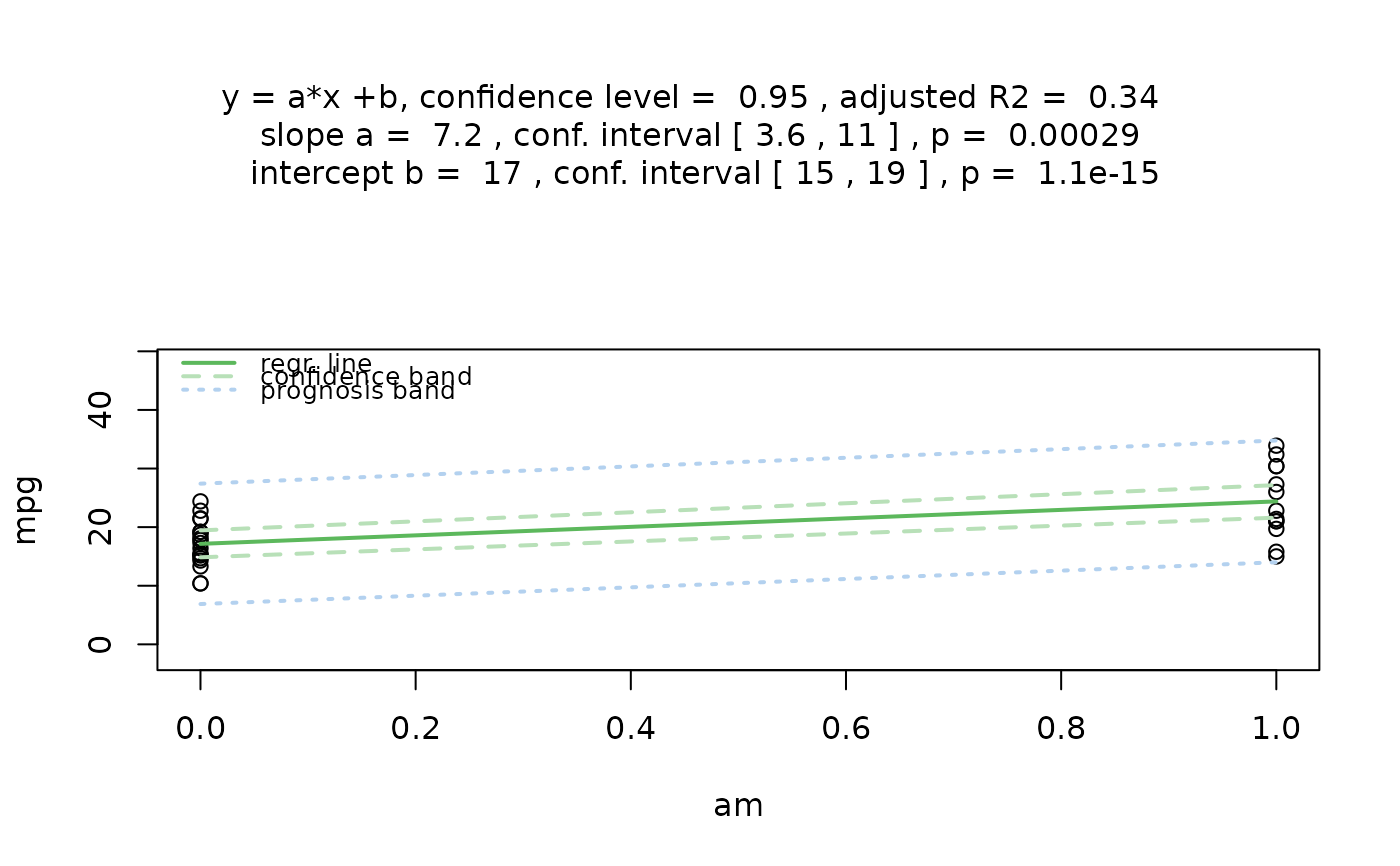
## Welch's t-test (unequal variances, two groups)
# When residuals are normally distributed but Levene's test indicates
# heteroscedasticity, Welch's t-test is used
visstat(mtcars$am, mtcars$mpg)




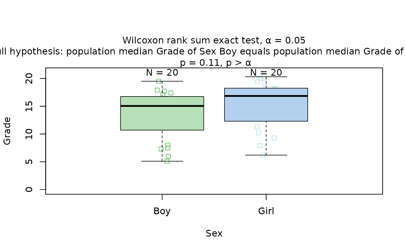
## Wilcoxon rank sum test (non-normal, two groups)
# When residuals are not normally distributed
grades_gender <- data.frame(
  Sex = as.factor(c(rep("Girl", 20), rep("Boy", 20))),
  Grade = c(
    19.3, 18.1, 15.2, 18.3, 7.9, 6.2, 19.4, 20.3, 9.3, 11.3,
    18.2, 17.5, 10.2, 20.1, 13.3, 17.2, 15.1, 16.2, 17.3, 16.5,
    5.1, 15.3, 17.1, 14.8, 15.4, 14.4, 7.5, 15.5, 6.0, 17.4,
    7.3, 14.3, 13.5, 8.0, 19.5, 13.4, 17.9, 17.7, 16.4, 15.6
  )
)
visstat(grades_gender$Sex, grades_gender$Grade)



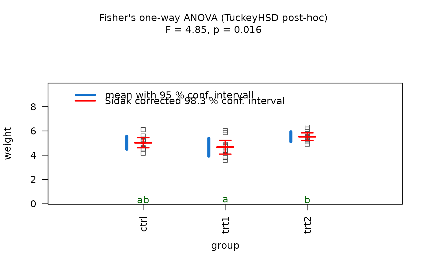
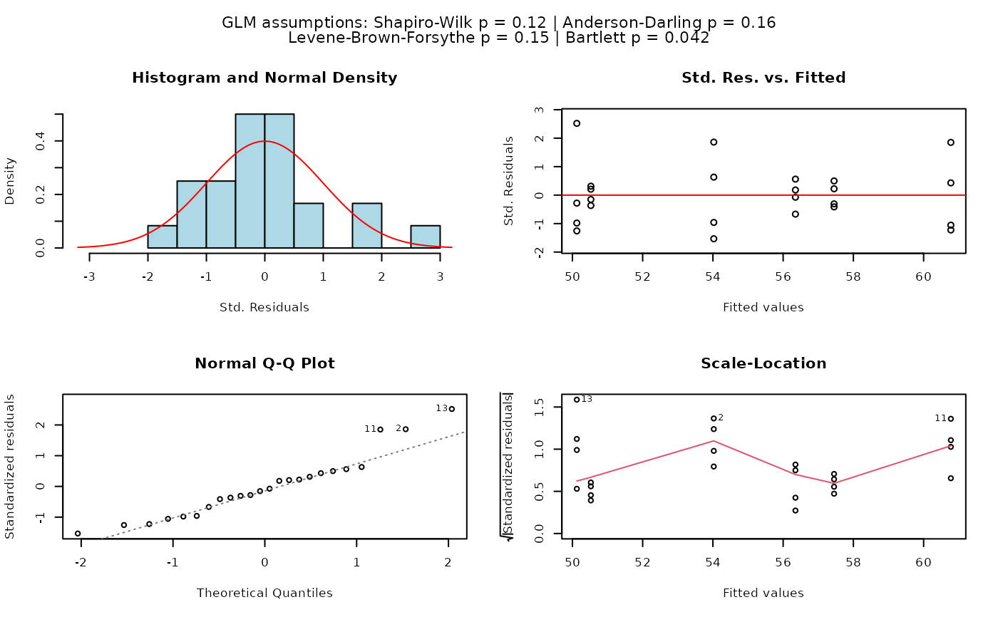
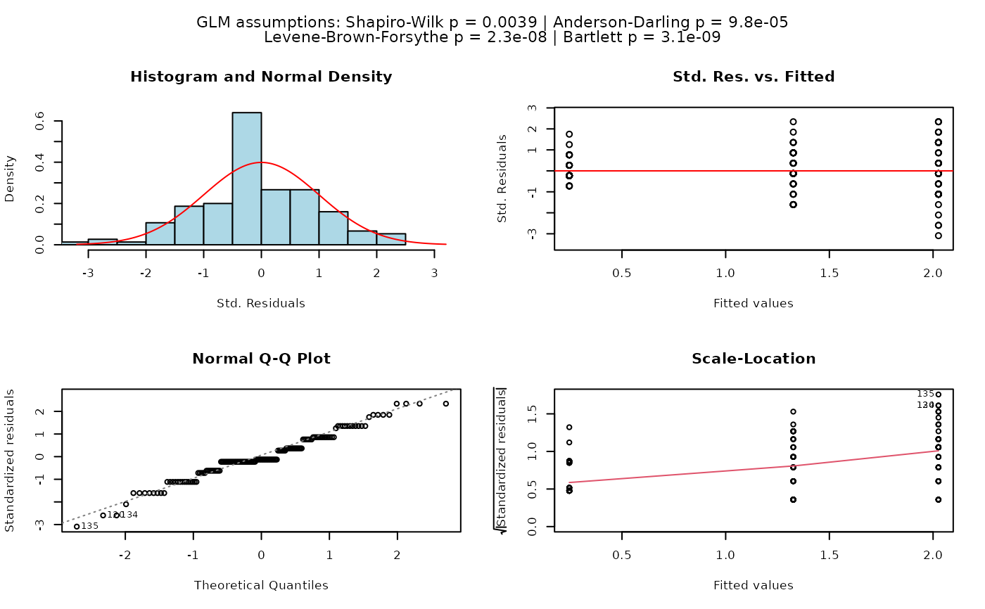
## Fisher's ANOVA (equal variances, >2 groups)
# When residuals are normally distributed and Levene's test indicates
# homoscedasticity, classic Fisher's ANOVA with TukeyHSD post-hoc is used.
# Different green letters indicate significant differences between groups. 
visstat(PlantGrowth$group, PlantGrowth$weight)



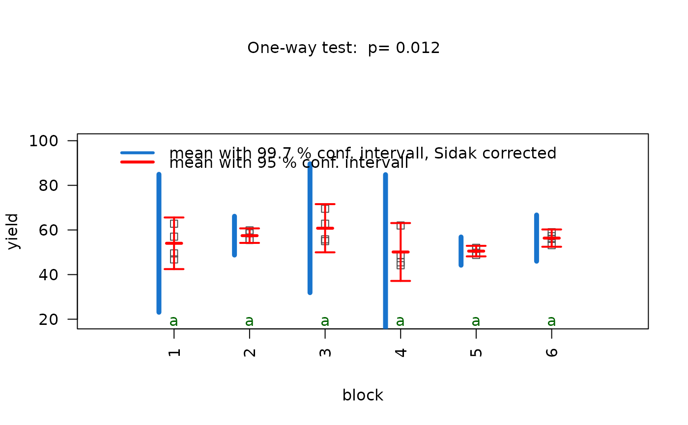
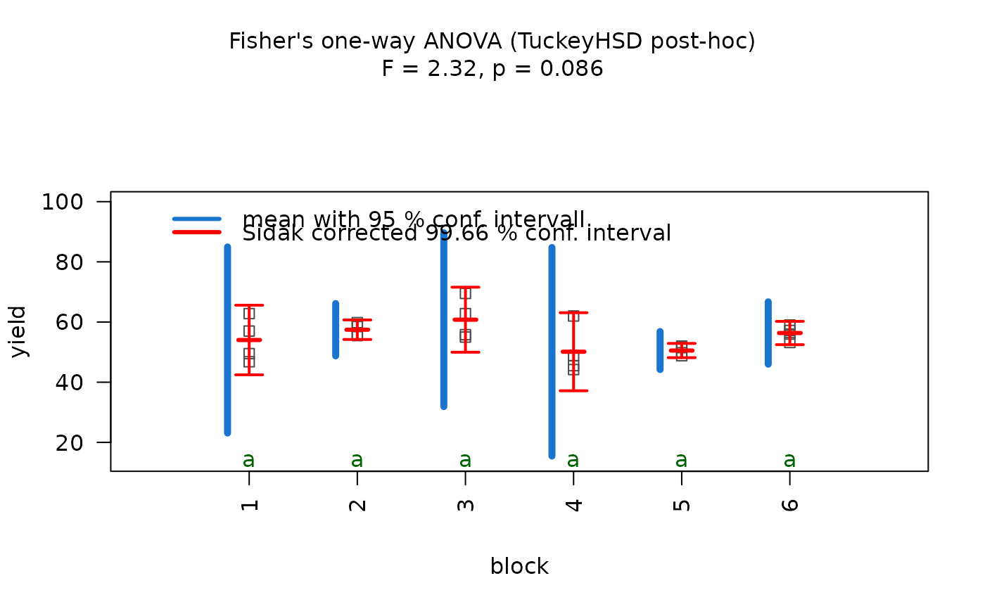
## Welch's one-way ANOVA (unequal variances, >2 groups)
set.seed(123)
values <- c(rnorm(20, 10, 1),rnorm(20, 15, 5),rnorm(20, 12, 2))
groups <- factor(rep(c("A", "B", "C"), each = 20))
visstat(groups, values)



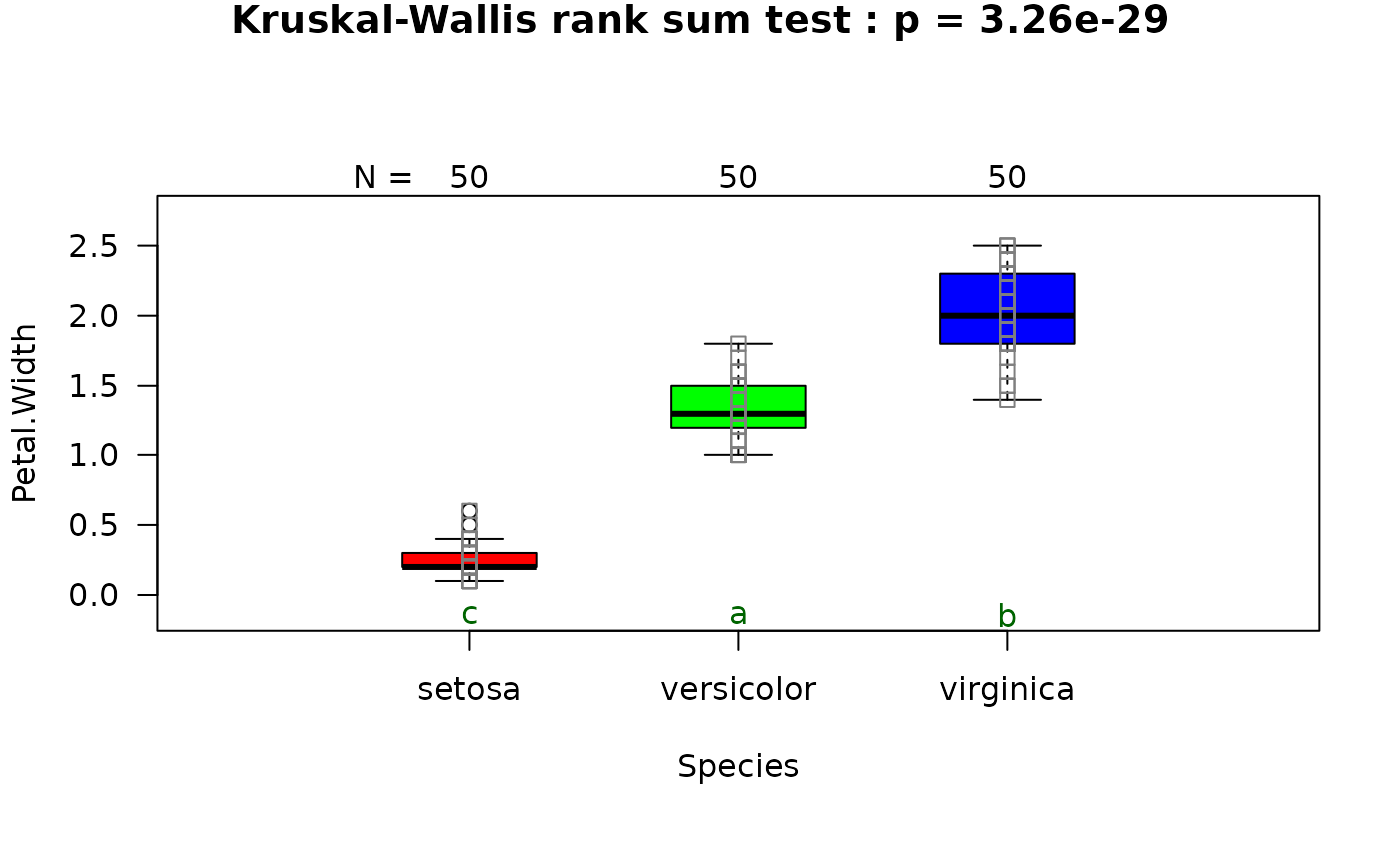
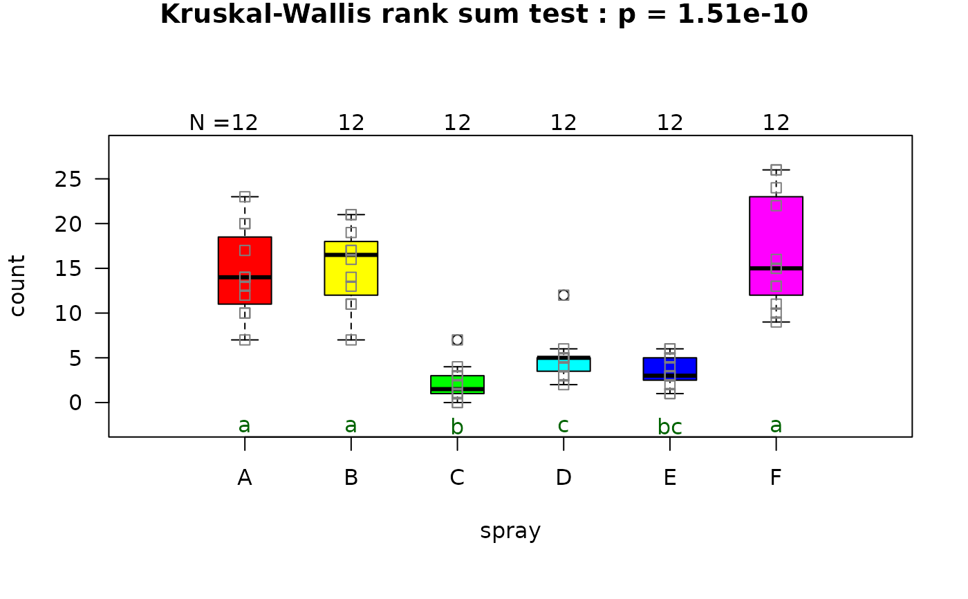
## Kruskal-Wallis (non-normal, >2 groups)
# When residuals are not normally distributed, kruskal.test() is followed by 
# pairwise.wilcox.test. 
visstat(iris$Species, iris$Petal.Width)



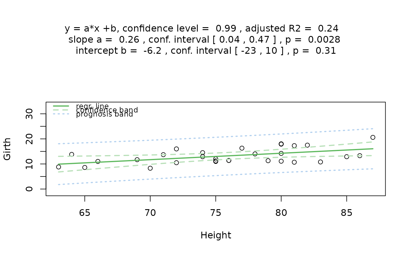
## Simple linear regression (both numeric)
visstat(trees$Height, trees$Girth, conf.level = 0.99)



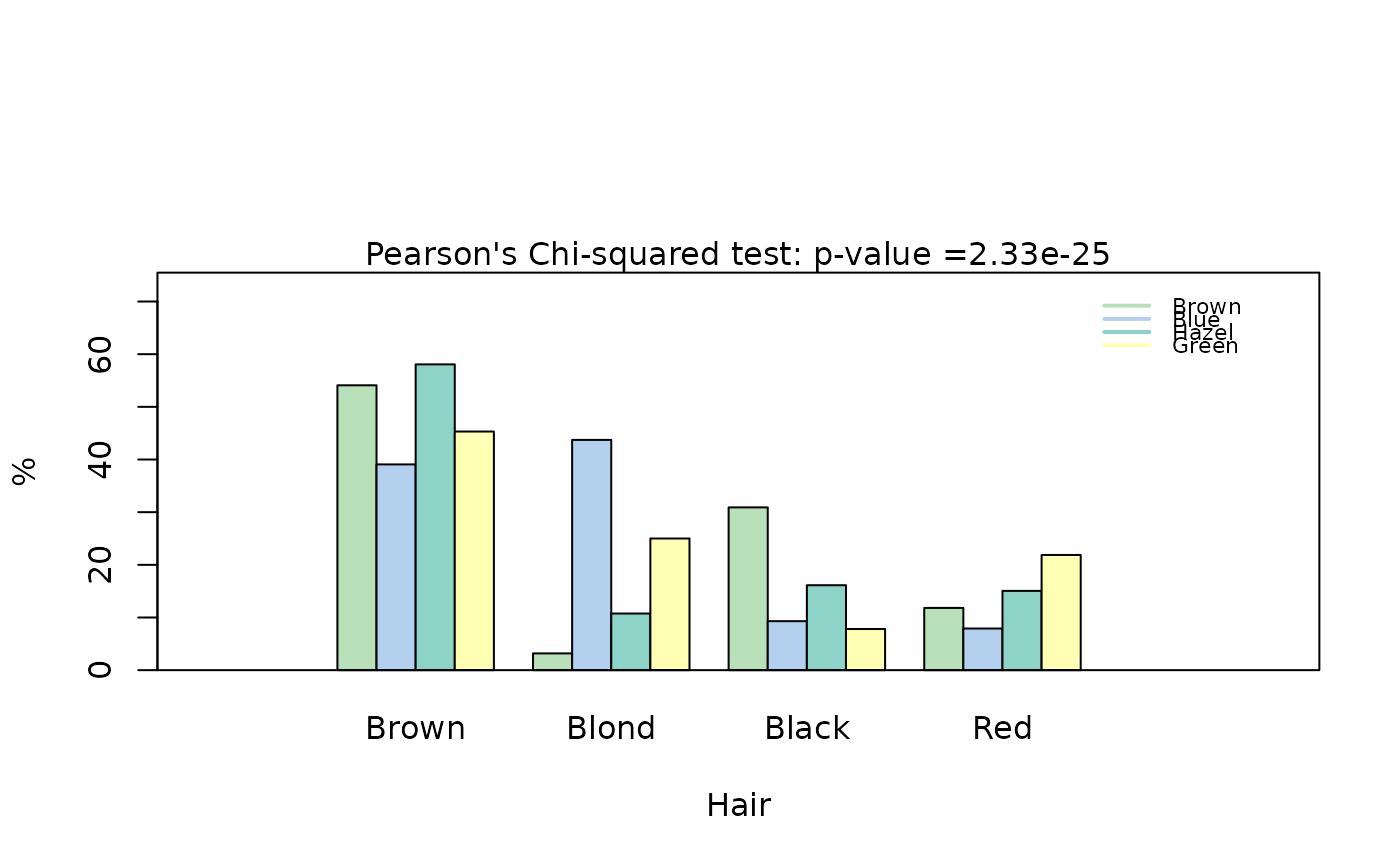
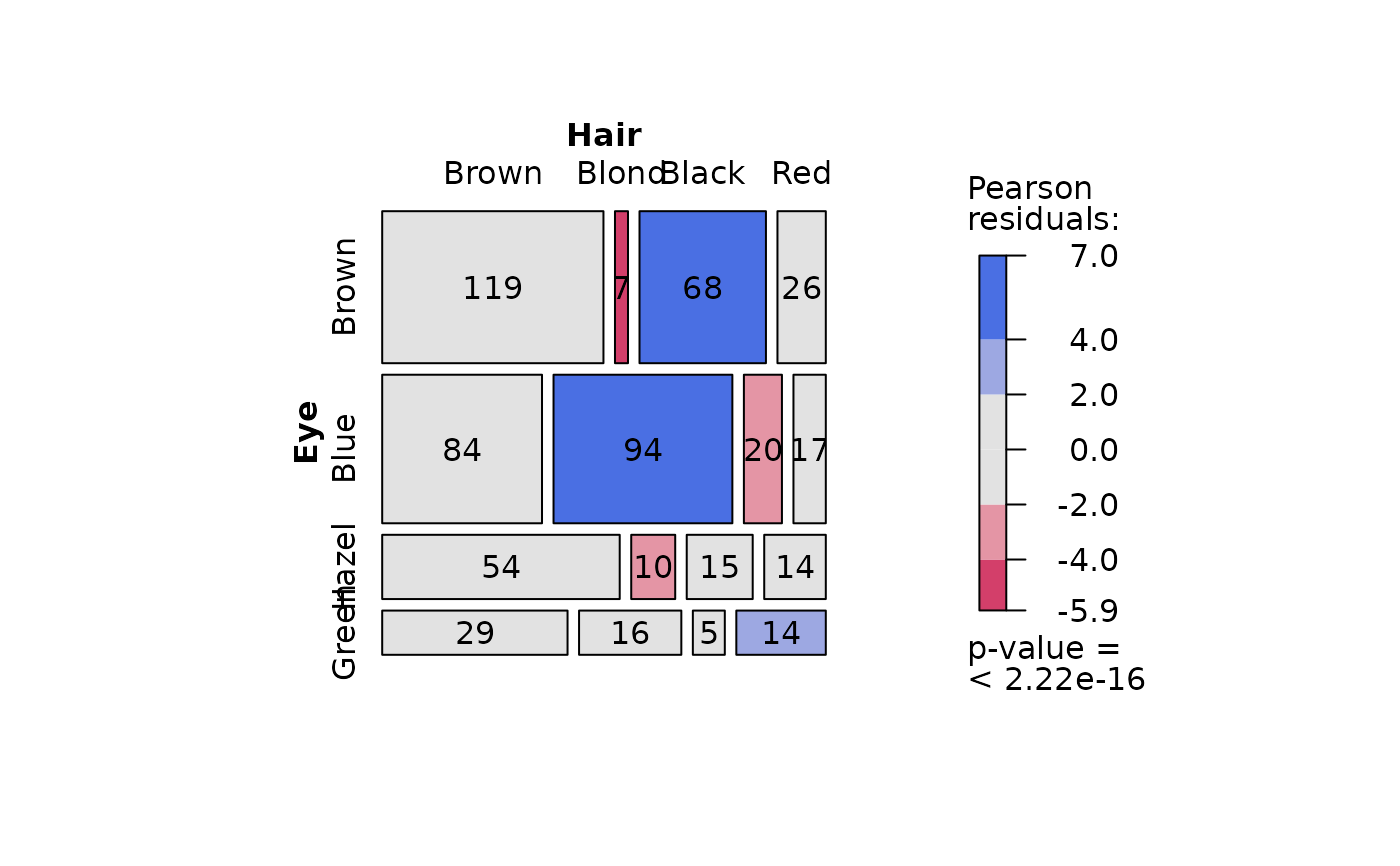
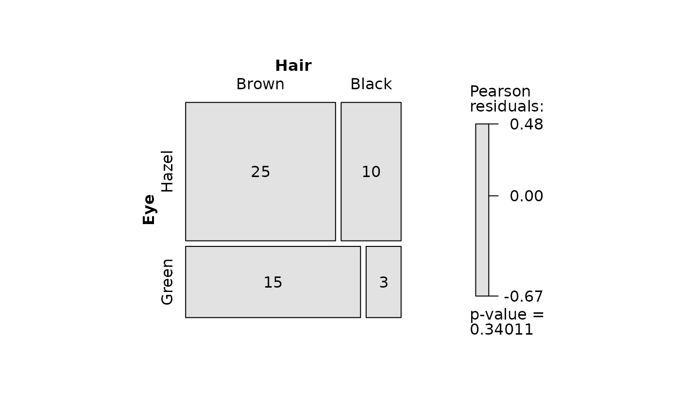
## Pearson's Chi-squared test (both factors, large expected counts)
HairEyeColorDataFrame <- counts_to_cases(as.data.frame(HairEyeColor))
visstat(HairEyeColorDataFrame$Eye, HairEyeColorDataFrame$Hair)



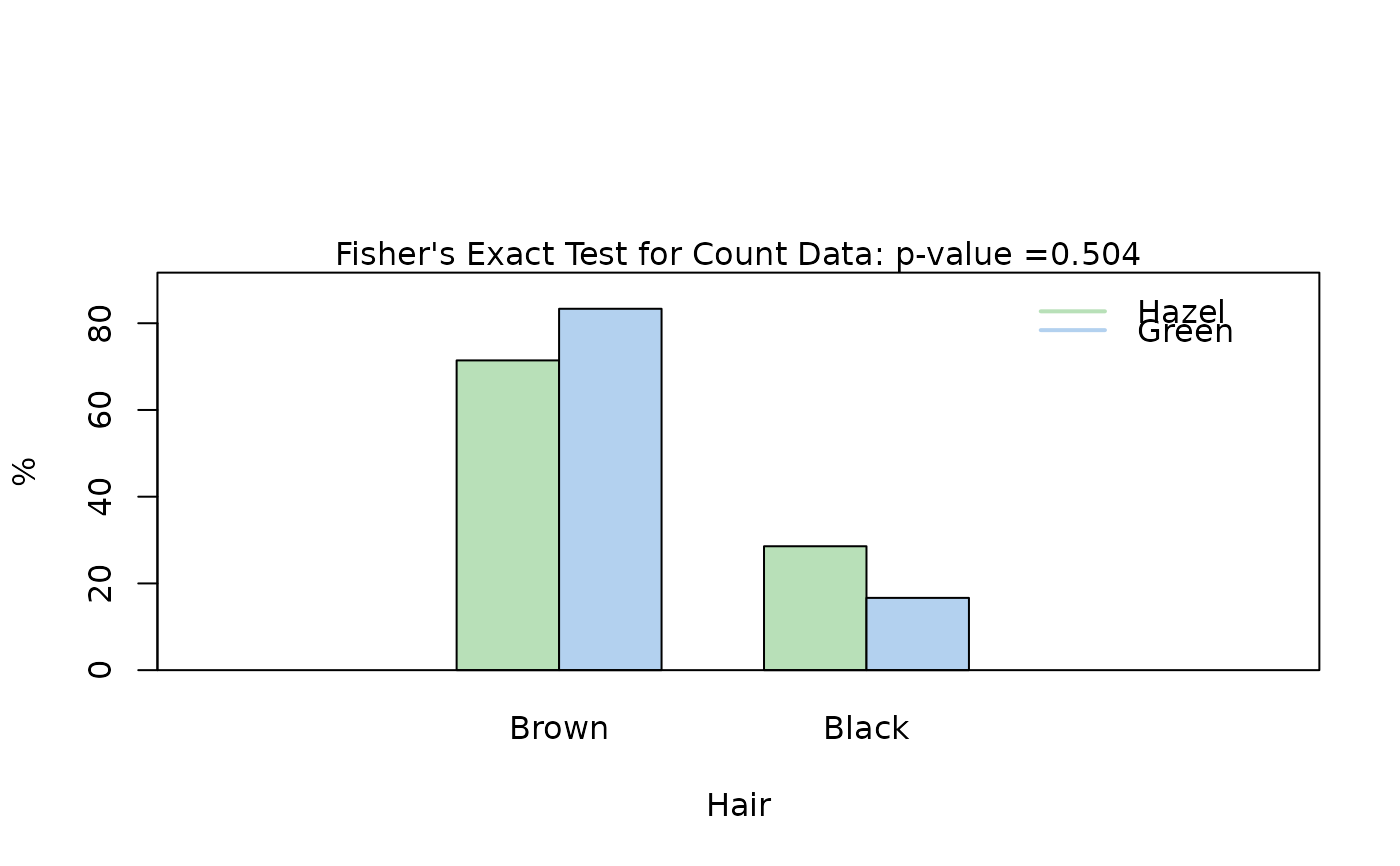
## Fisher's exact test (both factors, small expected counts)
HairEyeColorMaleFisher <- HairEyeColor[, , 1]
blackBrownHazelGreen <- HairEyeColorMaleFisher[1:2, 3:4]
blackBrownHazelGreen <- counts_to_cases(as.data.frame(blackBrownHazelGreen))
visstat(blackBrownHazelGreen$Eye, blackBrownHazelGreen$Hair)



## Save PNG
visstat(blackBrownHazelGreen$Hair, blackBrownHazelGreen$Eye,
        graphicsoutput = "png", plotDirectory = tempdir())

## Custom plot name
visstat(iris$Species, iris$Petal.Width,
        graphicsoutput = "pdf", plotName = "kruskal_iris", plotDirectory = tempdir())
#> Warning: calling par(new=TRUE) with no plot